Univariate data - Geospatial

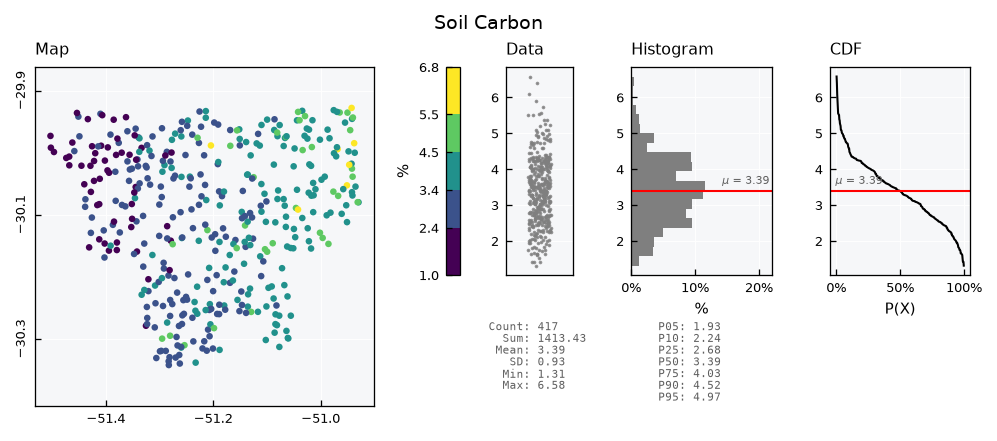
This tutorial covers the GeoUnivar object, a Univar whose values have a location. It adds a map panel to the standard visual, next to the data, the histogram and the CDF.

See also

Check out the Univariate data - Basics and Univariate data - Plots tutorials first.

Notebook setup

For users running this tutorial as a Jupyter Notebook, this cell must be executed first:

import sys
from pathlib import Path
import numpy as np
import matplotlib.pyplot as plt
import geopandas as gpd
from shapely.geometry import Polygon

# Install `plans` in `google.colab`.
# Use `pip install plans` for other environments.

if "google.colab" in sys.modules:
    import os
    os.system(f"{sys.executable} -m pip install -q plans")

from plans.datasets.analyst import GeoUnivar
from plans.stochastic.binning import get_bins

# This avoids warnings related to uninstalled fonts
import logging
# Set the matplotlib font manager logger to only show errors (hides warnings)
logging.getLogger('matplotlib.font_manager').setLevel(logging.ERROR)

# define output folder
OUTPUT_DIR = Path("outputs/geounivar")
OUTPUT_DIR.mkdir(parents=True, exist_ok=True)
print(f"Outputs will be saved to: ./{OUTPUT_DIR}")

Outputs will be saved to: ./outputs/geounivar

Sample data

Lets make all the data from scratch with geopandas, using geographic coordinates. First, a catchment, as a single polygon. Its outline is a circle, with a radius that varies around the center:

rng = np.random.default_rng(seed=1)  # ensure reproducibility

angle = np.linspace(start=0, stop=2 * np.pi, num=60, endpoint=False)
radius = 0.2 + 0.05 * np.sin(3 * angle) + 0.025 * np.cos(7 * angle + 1)
x = -51.2 + 1.3 * radius * np.cos(angle)
y = -30.1 + radius * np.sin(angle)

catchment = gpd.GeoDataFrame(
    data={"name": ["Catchment"]},
    geometry=[Polygon(shell=list(zip(x, y)))],
    crs="EPSG:4674",
)
catchment

	name	geometry
0	Catchment	POLYGON ((-50.92244 -30.1, -50.92667 -30.0779,...

Next, the points: soil samples at random locations. They are drawn over the bounding box of the catchment, and only those within the polygon are kept:

xmin, ymin, xmax, ymax = catchment.total_bounds

points = gpd.GeoDataFrame(
    geometry=gpd.points_from_xy(
        x=rng.uniform(low=xmin, high=xmax, size=600),
        y=rng.uniform(low=ymin, high=ymax, size=600),
        crs="EPSG:4674",
    )
)
points = points[points.within(other=catchment.geometry.iloc[0])].reset_index(drop=True)
print(f"{len(points)} points")

417 points

Each sample gets a value of soil organic carbon. Values rise to the east, with some skewed noise, so the map has a pattern to show:

east = (points.geometry.x - xmin) / (xmax - xmin)
points["soc"] = 1 + 3 * east + rng.gamma(shape=2, scale=0.4, size=len(points))
points.head()

	geometry	soc
0	POINT (-51.20624 -30.24392)	3.770107
1	POINT (-51.42191 -30.01331)	1.750928
2	POINT (-50.94999 -29.93546)	5.514472
3	POINT (-51.32355 -30.2484)	3.417389
4	POINT (-51.25815 -30.27589)	2.367847

Setting the data

A GeoUnivar holds a GeoDataFrame in its .data attribute. The .set_data() method takes the GeoDataFrame and the name of the column of values. It keeps only the values and the geometry, in a new table, and drops rows with missing values:

gv = GeoUnivar(name="Soil Carbon", alias="SOC")
gv.varname = "Soil Organic Carbon"
gv.units = "%"
gv.set_data(input_df=points, input_varfield="soc")
gv.data.head()

	v	geometry
0	3.770107	POINT (-51.20624 -30.24392)
1	1.750928	POINT (-51.42191 -30.01331)
2	5.514472	POINT (-50.94999 -29.93546)
3	3.417389	POINT (-51.32355 -30.2484)
4	2.367847	POINT (-51.25815 -30.27589)

Statistics work as in Univar:

gv.stats_df

	statistic	value
0	count	417.000000
1	sum	1413.427918
2	mean	3.389515
3	sd	0.929507
4	min	1.312094
5	p01	1.538221
6	p05	1.932009
7	p10	2.237571
8	p20	2.550812
9	p25	2.684995
10	p40	3.118546
11	p50	3.391361
12	p60	3.590346
13	p75	4.032204
14	p80	4.168357
15	p90	4.523499
16	p95	4.967135
17	p99	5.698861
18	max	6.581758

Standard visualization

Get the standard visual using the .view() method. Colors on the map follow classes of value, shown on the color bar, with labels at the boundaries of the classes. The bar holds the y axis of the panels at its right, so a value is at the same height on all of them. For this, the outer classes reach the ends of the range of the panels. The map panel is always square and aligned with the top of the other panels, so its view limits widen to fit the shape of the data:

gv.view()

GeoUnivar has two layouts:

print(gv.layouts.keys())

dict_keys(['full', 'mini'])

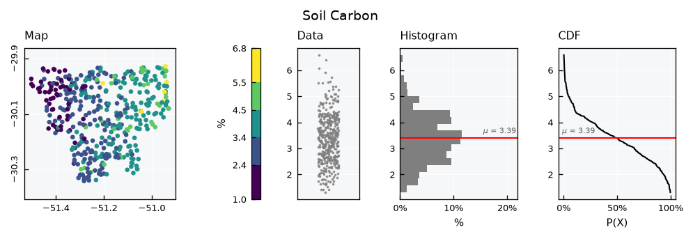
The mini layout has a smaller map and drops the statistics table:

gv.view_specs["layout"] = "mini"
gv.view()

Color schemes

Colors follow classes of value, five by default, and the scheme_cmap key sets how they are defined. There are two options for classes, and get_bins() shows the boundaries each one gives for this sample:

vct_values = gv.data[gv.varfield].values
for scheme in ["equal", "quantiles"]:
    bins = get_bins(data=vct_values, n_bins=5, scheme=scheme)
    print(f"{scheme:>9}: {np.round(bins, 2)}")

    equal: [1.31 2.37 3.42 4.47 5.53 6.58]
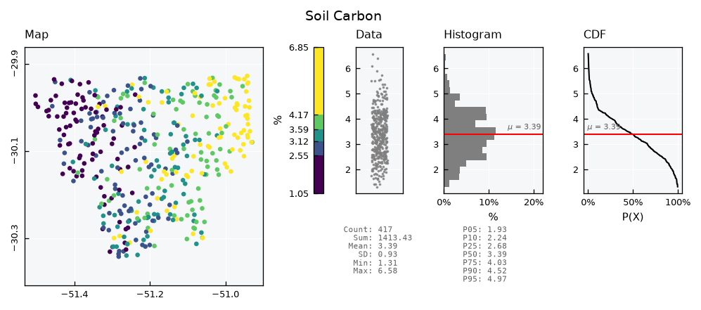
quantiles: [1.31 2.55 3.12 3.59 4.17 6.58]

equal is the default, with classes of the same width. It keeps the scale of the values, so high values stand out, but most points fall in the middle classes:

gv.view_specs["layout"] = "full"
gv.view_specs["scheme_cmap"] = "equal"
gv.view()

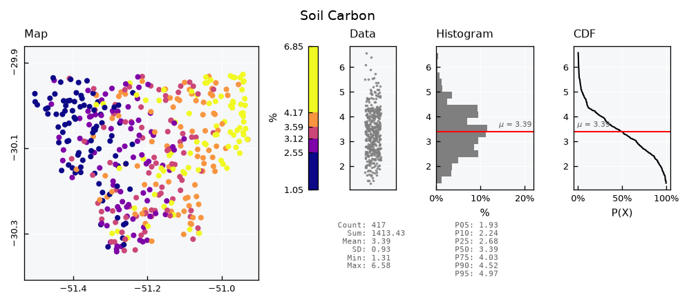
quantiles makes classes with the same number of points. All colors are used evenly, so the west to east pattern is clearer, but classes have different widths, as the color bar shows:

gv.view_specs["scheme_cmap"] = "quantiles"
gv.view()

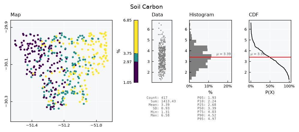
The n_classes_cmap key sets the number of classes. Fewer classes give a simpler map, and the color bar follows:

gv.view_specs["n_classes_cmap"] = 3
gv.view()

The cmap key sets the colors, with any matplotlib color map name. Other map options are the keys ending in _map, such as marker_map and markersize_map:

gv.view_specs["n_classes_cmap"] = 5
gv.view_specs["cmap"] = "plasma"
gv.view_specs["markersize_map"] = 15
gv.view()

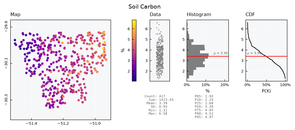
With scheme_cmap as continuous, colors change smoothly instead of by classes. The scale spans the range key, the same as the y axis of the other panels, so a fixed range also fixes the colors:

gv.view_specs["scheme_cmap"] = "continuous"
gv.view()

The color bar

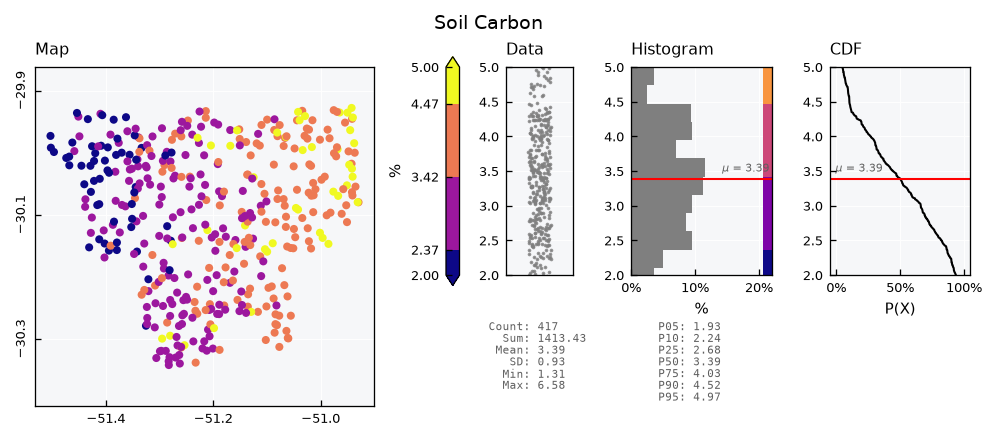
If the range key clips the data, a triangular tip on the color bar marks that side, to show that the data continues. Here, the range cuts both ends. The cbar_map key removes the bar altogether, and strips inside the data and histogram panels are available with the cbar_scatter and cbar_histh keys:

gv.view_specs["scheme_cmap"] = "equal"
v_range = gv.view_specs["range"]
gv.view_specs["range"] = [2, 5]
gv.view_specs["cbar_histh"] = True
gv.view()

Adding the catchment

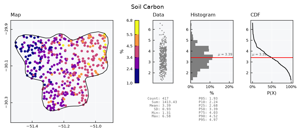
The helper_geometry key overlays one GeoDataFrame, in the same CRS as the points. By default, it is an outline above the data:

gv.view_specs["range"] = v_range
gv.view_specs["cbar_histh"] = False
gv.view_specs["helper_geometry"] = catchment
gv.view()

The keys ending in _helper set its style. A filled polygon needs a zorder_helper below zorder_map, to stay under the points:

gv.view_specs["facecolor_helper"] = "gainsboro"
gv.view_specs["zorder_helper"] = 1
gv.view()

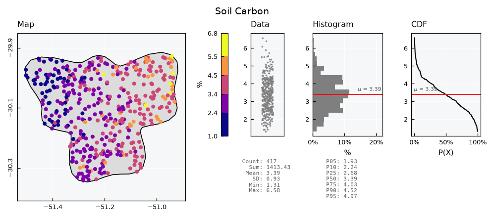
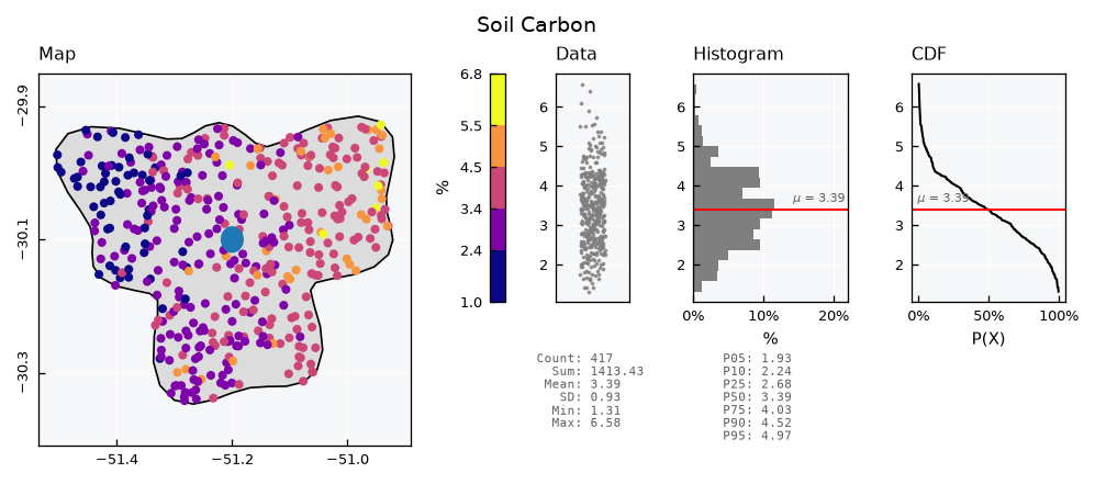
For any other geometry, get the figure with return_fig=True and plot on the map axis, which is the first one:

lake = gpd.GeoDataFrame(
    geometry=gpd.points_from_xy(x=[-51.2], y=[-30.1]).buffer(distance=0.02),
    crs="EPSG:4674",
)

fig = gv.view(show=False, return_fig=True)
ax_map = fig.get_axes()[0]
lake.plot(ax=ax_map, facecolor="tab:blue", edgecolor="none", zorder=5)
ax_map.set(xlabel="", ylabel="")  # recent versions of geopandas add labels
plt.show()

Loading from a file

The data usually comes from a file. Lets write both layers to a GeoPackage:

file_db = OUTPUT_DIR / "catchment.gpkg"
points.to_file(filename=file_db, layer="samples", driver="GPKG")
catchment.to_file(filename=file_db, layer="catchment", driver="GPKG")

The .load_data() method takes the file, the name of the layer and the name of the column of values, and gives the same table as .set_data():

gv_file = GeoUnivar(name="Soil Carbon", alias="SOC")
gv_file.varname = "Soil Organic Carbon"
gv_file.units = "%"
gv_file.load_data(file_data=file_db, layer_name="samples", input_varfield="soc")
gv_file.data.head()

	v	geometry
0	3.770107	POINT (-51.20624 -30.24392)
1	1.750928	POINT (-51.42191 -30.01331)
2	5.514472	POINT (-50.94999 -29.93546)
3	3.417389	POINT (-51.32355 -30.2484)
4	2.367847	POINT (-51.25815 -30.27589)

Other layers, like the catchment, are read with geopandas itself:

catchment_file = gpd.read_file(filename=file_db, layer="catchment")
catchment_file

	name	geometry
0	Catchment	POLYGON ((-50.92244 -30.1, -50.92667 -30.0779,...

Recap

• GeoUnivar is a Univar with a GeoDataFrame as data, and a map panel in its visual.

• .set_data() and .load_data() take the name of the column of values.

• view_specs["layout"] switches between full and mini.

• scheme_cmap defines the colors, as classes by equal or quantiles, or as continuous. n_classes_cmap sets how many classes, and cmap sets the colors.

• The color bar has a tip where range clips the data. cbar_map removes it, and the _map keys set the map panel.

• helper_geometry adds one geometry to the map, and the figure takes any others.