Bivariate data - Basics

This tutorial focuses on working with paired (bivariate) data using plans: loading x/y samples, visualizing their joint distribution and measuring their agreement with standard metrics.

Notebook setup

For users running this tutorial as a Jupyter Notebook, this cell must be executed first:

import sys
from pathlib import Path
import numpy as np
import pandas as pd

# Install `plans` in `google.colab`.
# Use `pip install plans` for other environments.

if "google.colab" in sys.modules:
    import os
    os.system(f"{sys.executable} -m pip install -q plans")

# This avoids warnings related to uninstalled fonts
import logging
# Set the matplotlib font manager logger to only show errors (hides warnings)
logging.getLogger('matplotlib.font_manager').setLevel(logging.ERROR)

# define output folder
OUTPUT_DIR = Path("outputs/bivariate")
OUTPUT_DIR.mkdir(parents=True, exist_ok=True)
print(f"Outputs will be saved to: ./{OUTPUT_DIR}")

Outputs will be saved to: ./outputs/bivariate

The Bivar object

The Bivar object lives under the plans.datasets.analyst module. Like Univar, it is a child of the DataSet object from plans.root, so it shares the same lifecycle: create the object, feed it data, and let .update() refresh the derived attributes.

See also

Check out the Univariate data - Basics tutorial first.

Import Bivar object:

from plans.datasets.analyst import Bivar

Create an instance of the Bivar:

bv = Bivar(name="Discharge", alias="Q")

Check out the variable type:

print(type(bv))

<class 'plans.datasets.analyst.Bivar'>

Handle data attributes

Columns are named by .xfield and .yfield, while .xname, .yname, .xunits and .yunits are only used as labels in visuals and metadata. Set labels before loading data, so the axis labels are built from them:

bv.description = "Observed and simulated daily discharge for a tutorial"
bv.xname = "Observed"
bv.xunits = "m3/s"
bv.yname = "Simulated"
bv.yunits = "m3/s"
print(f"x column: {bv.xfield} | y column: {bv.yfield}")

x column: x | y column: y

Working with data

Create synthetic dataset

A common bivariate case in hydrology is comparing observed against simulated discharge. Lets make one year of skewed daily observations and a simulation that slightly overestimates them with some noise. A couple of values are missing.

# make synthetic data
rng = np.random.default_rng(seed=42)  # ensure reproducibility
q_obs = rng.gamma(shape=2, scale=10, size=365)
q_sim = 1.05 * q_obs + rng.normal(loc=0, scale=3, size=len(q_obs))
q_sim = np.clip(q_sim, a_min=0, a_max=None)
df = pd.DataFrame({"q_obs": q_obs, "q_sim": q_sim})
df.loc[[3, 7], "q_sim"] = np.nan

# Export CSV file
file_csv = OUTPUT_DIR / "bivariate_discharge.csv"
df.to_csv(file_csv, sep=";", index=False)
print(f"Saved to: {file_csv}")
df.head()

Saved to: outputs/bivariate/bivariate_discharge.csv

	q_obs	q_sim
0	20.918173	15.121868
1	28.353456	25.281213
2	18.372156	16.522104
3	16.450704	NaN
4	30.792553	33.179942

Loading data from the CSV file

Call the .load_data() method, pointing which file columns hold x and y. They are renamed to .xfield and .yfield on loading:

bv.load_data(
    file_data=file_csv,  # file path
    input_xfield="q_obs",  # name of x column
    input_yfield="q_sim",  # name of y column
    in_sep=";",  # input separator
)

Data is stored in the .data attribute as a pandas.DataFrame. Incomplete pairs are dropped and rows are sorted by x:

bv.data

	x	y
0	0.927625	4.918430
1	1.046498	0.402015
2	1.073776	0.000000
3	1.474360	7.263258
4	1.513774	3.123128
...	...	...
358	68.394419	73.005240
359	70.228886	71.807229
360	71.510124	73.848619
361	74.869975	75.930436
362	89.335951	96.356605

363 rows × 2 columns

Tip

For in-memory arrays, use .set_data(x=..., y=...) instead. It applies the same cleaning and sorting.

Access computed attributes

After loading data, some attributes are computed automatically:

print(f"Size: {bv.size}")
print(f"x range: {bv.x_min:.2f} to {bv.x_max:.2f}")
print(f"y range: {bv.y_min:.2f} to {bv.y_max:.2f}")

Size: 363
x range: 0.93 to 89.34
y range: 0.00 to 96.36

Inspect the object metadata:

bv.get_metadata()

{'name': 'Discharge',
 'alias': 'Q',
 'size': 363,
 'color': 'blue',
 'source': None,
 'description': 'Observed and simulated daily discharge for a tutorial',
 'xunits': 'm3/s',
 'yunits': 'm3/s',
 'file_data': '/home/runner/work/plans/plans/docs/tutorials/outputs/bivariate/bivariate_discharge.csv'}

Visualizations

Standard visualization

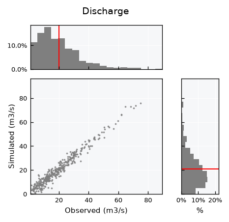
Get the standard visual using the .view() method. The full layout shows the scatter plot with the marginal histograms of x (top) and y (right):

bv.view()

Fine-tuning visuals

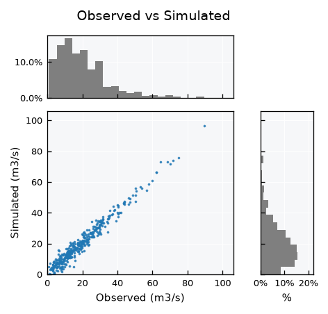
Like other plans objects, use the .view_specs keys for fine tuning. When comparing the same variable, equal axis ranges make the plot easier to read:

q_max = 1.1 * max(bv.x_max, bv.y_max)
bv.view_specs["range_x"] = [0, q_max]
bv.view_specs["range"] = [0, q_max]
bv.view_specs["color"] = "tab:blue"
bv.view_specs["bins"] = 20  # default None uses the Freedman-Diaconis rule
bv.view_specs["plot_mean"] = False
bv.view_specs["title"] = "Observed vs Simulated"
bv.view()

See also

The model layout for model assessment is covered in the Bivariate data - Models tutorial.

Metrics

All metrics are static methods, so they can be used on any pair of arrays. Correlations are symmetric and take any two variables x and y:

• Pearson \(r\) measures linear association.

• Spearman \(\rho\) is the Pearson \(r\) of the ranks, so it measures monotonic association. It reaches 1 for any increasing relation, linear or not.

Agreement metrics are not symmetric and take an observed and a predicted series of the same variable:

• Coefficient of determination \(R^2 = 1 - SS_{res} / SS_{tot}\) is the fraction of observed variance explained by the predictions. It is negative when the predictions are worse than the observed mean.

• RMSE, MAE and Bias (%) measure the error magnitude and its direction. Bias is positive when the predictions overestimate.

obs = bv.data[bv.xfield].values
sim = bv.data[bv.yfield].values

print(f"r: {Bivar.pearson(x=obs, y=sim):.3f}")
print(f"rho: {Bivar.spearman(x=obs, y=sim):.3f}")
print(f"R2: {Bivar.rsq(observed=obs, predicted=sim):.3f}")
print(f"RMSE: {Bivar.rmse(observed=obs, predicted=sim):.3f}")
print(f"MAE: {Bivar.mae(observed=obs, predicted=sim):.3f}")
print(f"Bias (%): {Bivar.bias(observed=obs, predicted=sim):.3f}")

r: 0.981

rho: 0.963
R2: 0.951
RMSE: 3.138
MAE: 2.506
Bias (%): 5.187

Or get them all at once with Bivar.get_metrics():

Bivar.get_metrics(observed=obs, predicted=sim)

{'r': 0.9806092604096887,
 'rho': 0.9631908543435195,
 'R2': 0.9511562724941502,
 'RMSE': 3.138448669315695,
 'MAE': 2.5062203403528733,
 'Bias': 5.18716362862958}

Association versus agreement

To see how metrics differ, compare our simulation with two noiseless but distorted ones: a doubled series (\(2 \cdot obs\)) and a curved series, still increasing but no longer a straight line:

sim_doubled = 2 * obs
sim_curved = 20 * np.power(obs / 20, 1.5)

df_metrics = pd.DataFrame(
    {
        "simulated": Bivar.get_metrics(observed=obs, predicted=sim),
        "doubled": Bivar.get_metrics(observed=obs, predicted=sim_doubled),
        "curved": Bivar.get_metrics(observed=obs, predicted=sim_curved),
    }
).T
df_metrics

	r	rho	R2	RMSE	MAE	Bias
simulated	0.980609	0.963191	0.951156	3.138449	2.506220	5.187164
doubled	1.000000	1.000000	-1.980150	24.514875	19.982952	100.000000
curved	0.980011	1.000000	0.216667	12.568511	6.040198	17.567995

Both distortions keep the ranks, so \(\rho = 1\). The doubled series is still a straight line, so \(r = 1\) as well, and the curved one stays close to it. Yet both have a much lower \(R^2\) than the noisy simulation: correlations measure association (how well some line or curve relates the series), while \(R^2\) and the error metrics measure agreement with the 1:1 line.