Univariate data - the basics

This tutorial focuses on working with basic univariate data management and analysis using plans.

Notebook setup

For users running this tutorial as a Jupyter Notebook, this cell must be executed first:

import sys
from pathlib import Path
import pprint
import numpy as np
import pandas as pd
import matplotlib.pyplot as plt

# Install `plans` in `google.colab`.
# Use `pip install plans` for other environments.

if "google.colab" in sys.modules:
    import os
    os.system(f"{sys.executable} -m pip install -q plans")

# This avoids warnings related to uninstalled fonts
import logging
# Set the matplotlib font manager logger to only show errors (hides warnings)
logging.getLogger('matplotlib.font_manager').setLevel(logging.ERROR)

# define output folder
OUTPUT_DIR = Path("outputs/univariate")
OUTPUT_DIR.mkdir(parents=True, exist_ok=True)
print(f"Outputs will be saved to: ./{OUTPUT_DIR}")

Outputs will be saved to: ./outputs/univariate

The Univar object

The Univar object is a very primitive class that lives under plans.analyst module. This object is a child from the DataSet object that lives in plans.root module.

The Univar stores all core methods for working with univariate data.

Import Univar object:

from plans.analyst import Univar

Create an instance of the Univar:

unv = Univar(name="Testing Univar", alias="uni-tst")

Check out the variable type:

print(type(unv))

<class 'plans.analyst.Univar'>

Handle data attributes

Inspect state for major attributes:

print(unv)

[Testing Univar (uni-tst)]
Univar (DS):	<class 'plans.analyst.Univar'>
      field          value
       name Testing Univar
      alias        uni-tst
       size            NaN
      color           blue
     source            NaN
description            NaN
      units          units
  file_data            NaN
Data:
None

Edit attributes directly and inspect again

unv.description = "A testing univariate for a tutorial"
unv.units = "cm"
print(unv)

[Testing Univar (uni-tst)]
Univar (DS):	<class 'plans.analyst.Univar'>
      field                               value
       name                      Testing Univar
      alias                             uni-tst
       size                                 NaN
      color                                blue
     source                                 NaN
description A testing univariate for a tutorial
      units                                  cm
  file_data                                 NaN
Data:
None

Working with data

Create synthetic gaussian dataset

Lets first make a synthetic gaussian dataset using numpy.random and save it to a CSV file using pandas.

# make synthetic gaussian data
np.random.seed(10) # ensure reproducibility
v = np.random.normal(loc=100, scale=10, size=1000)
df = pd.DataFrame({"variable": v})

# Export CSV file
file_csv = OUTPUT_DIR / "univariate_gauss.csv"
df.to_csv(file_csv, sep=";", index="False")
print(f"Saved to: {file_csv}")

Saved to: outputs/univariate/univariate_gauss.csv

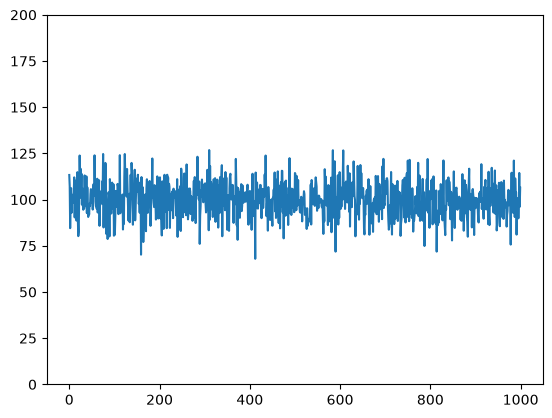
The whole dataset looks like this:

# get simple visualization
plt.plot(df.index, df['variable'])
plt.ylim([0, 200])
plt.show()

Loading data from the CSV file

Call the .load_data() method for loading from CSV file:

# reset the uv variable
unv = Univar(name="Testing Univar", alias="uni-tst")

unv.load_data(
    file_data=file_csv,  # file path
    input_varfield="variable",  # name of column/field
    in_sep=";",  # input separator
)

Data is stored in the .data attribute as a pandas.DataFrame:

unv.data

	v
0	113.315865
1	107.152790
2	84.545997
3	99.916162
4	106.213360
...	...
995	89.856608
996	96.681723
997	114.406974
998	96.097821
999	106.424506

1000 rows × 1 columns

Access computed metadata

After loading data, some useful attributes are computed automatically.

Basic statistics are stored in .stats_df as a pandas.DataFrame:

unv.stats_df

	statistic	value
0	count	1000.000000
1	sum	99854.433644
2	mean	99.854434
3	sd	9.379578
4	min	67.955987
5	p01	78.678389
6	p05	84.521828
7	p10	87.959449
8	p20	92.072856
9	p25	93.609900
10	p40	97.618150
11	p50	99.765252
12	p60	102.116821
13	p75	106.010132
14	p80	107.549608
15	p90	111.678248
16	p95	114.846091
17	p99	122.426391
18	max	126.799103

Data frequencies are stored in .freq_df as a pandas.DataFrame:

unv.freq_df

	Percentiles	Exceedance	Frequency	Empirical Probability	Values
0	0	100	1	0.001	67.955987
1	1	99	0	0.000	78.678389
2	2	98	0	0.000	80.584361
3	3	97	1	0.001	82.311344
4	4	96	0	0.000	83.409942
...	...	...	...	...	...
95	95	5	2	0.002	114.846091
96	96	4	2	0.002	116.115753
97	97	3	0	0.000	118.178726
98	98	2	0	0.000	120.658142
99	99	1	3	0.003	122.426391

100 rows × 5 columns

Data weibull CDF is stored in .weibull_df as a pandas.DataFrame:

unv.weibull_df

	Data	P(X)	F(X)
0	126.799103	0.000999	0.999001
1	126.716851	0.001998	0.998002
2	126.625775	0.002997	0.997003
3	124.676511	0.003996	0.996004
4	124.653251	0.004995	0.995005
...	...	...	...
995	74.885309	0.995005	0.004995
996	71.849387	0.996004	0.003996
997	71.839988	0.997003	0.002997
998	70.204032	0.998002	0.001998
999	67.955987	0.999001	0.000999

1000 rows × 3 columns

Visualizations

Most plans. objects comes with built-in methods for getting visualizations, both inline and figure output.

See also

Check out more about visualizations on the Visualizations - the basics tutorial.

Standard visualization

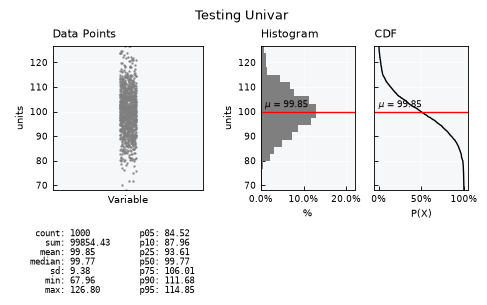
Get the standard visual using the .view() method

unv.view()

Fine-tuning visuals

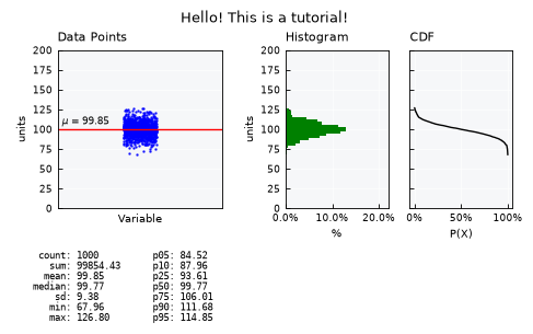
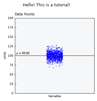
Use the .view_specs keys for fine tuning the visual. Example of some possibilities:

# Y axis range
unv.view_specs["range"] = [0, 200]
# Scatter
unv.view_specs["scatter_factor"] = 2 # occupy more space
# Color
unv.view_specs["color"] = "blue"
unv.view_specs["color_hist"] = "green"
# Decorations
unv.view_specs["plot_mean"] = False
unv.view_specs["plot_mean_data"] = True
unv.view_specs["title"] = "Hello! This is a tutorial!"
# call view again
unv.view()

Layouts available

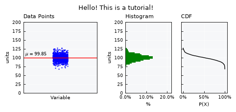
List available layout keys:

print(unv.layouts.keys())

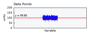
dict_keys(['full', 'mini', 'simple', 'simple-shallow', 'default'])

unv.view_specs["layout"] = "mini"
unv.view()

unv.view_specs["layout"] = "simple"
unv.view()

unv.view_specs["layout"] = "simple-shallow"
unv.view_specs["title"] = None
unv.view()

Analysis methods

Normality assessment

Assess if the data is normal via the .get_normality() method:

df = unv.get_normality(clevel=0.95)
df

	Test	Statistic	p-value	is_normal	Confidence
0	Kolmogorov-Smirnov	0.013838	0.989545	True	0.95
1	Shapiro-Wilk	0.998710	0.695039	True	0.95
2	D'Agostino-Pearson	0.477945	0.787436	True	0.95

Weibull distribution

df = unv.get_cdf_weibull()
df

	Data	P(X)	F(X)
0	126.799103	0.000999	0.999001
1	126.716851	0.001998	0.998002
2	126.625775	0.002997	0.997003
3	124.676511	0.003996	0.996004
4	124.653251	0.004995	0.995005
...	...	...	...
995	74.885309	0.995005	0.004995
996	71.849387	0.996004	0.003996
997	71.839988	0.997003	0.002997
998	70.204032	0.998002	0.001998
999	67.955987	0.999001	0.000999

1000 rows × 3 columns

Gumbel distribution

The method .get_cdf_gumbel() performs a full assessment for the Gumbel distribution.

Warning

This method assumes the data is a collection of maxima values.

dc_gumbel = unv.get_cdf_gumbel()

View model results:

df = dc_gumbel["Metadata"]
df

	Metadata	Value
0	N	1000
1	Gumbel a	95.633125
2	Gumbel b	7.313227
3	KS-test s-value	0.076734
4	KS-test p-value	0.000014
5	KS-test Is Gumbel (NullH)	False
6	QQ-plot c0	2.405764
7	QQ plot c1	0.975998
8	QQ-plot r2	0.970525

View data:

df = dc_gumbel["Data"]
df

	v	Rank	P(X)_Empirical	P(X)_Weibull	T(X)_Weibull	P(X)_Gringorten	P(X)_Gumbel	T(X)_Gumbel	T(X)_Gumbel_SE90	T(X)_Gumbel_P05	T(X)_Gumbel_P95
0	126.799103	1	0.001	0.000999	1001.000000	0.000560	0.014001	71.423884	1.784416	56.068652	91.022575
1	126.716851	2	0.002	0.001998	500.500000	0.001560	0.014158	70.630695	1.780045	55.480053	89.956708
2	126.625775	3	0.003	0.002997	333.666667	0.002560	0.014334	69.762759	1.775206	54.835575	88.791140
3	124.676511	4	0.004	0.003996	250.250000	0.003560	0.018671	53.557703	1.671825	42.715790	67.184470
4	124.653251	5	0.005	0.004995	200.200000	0.004559	0.018730	53.389231	1.670594	42.588833	66.961535
...	...	...	...	...	...	...	...	...	...	...	...
995	74.885309	996	0.996	0.995005	1.005020	0.995441	1.000000	1.000000	1.172041	1.000000	1.000000
996	71.849387	997	0.997	0.996004	1.004012	0.996440	1.000000	1.000000	1.328611	1.000000	1.000000
997	71.839988	998	0.998	0.997003	1.003006	0.997440	1.000000	1.000000	1.329099	1.000000	1.000000
998	70.204032	999	0.999	0.998002	1.002002	0.998440	1.000000	1.000000	1.414199	1.000000	1.000000
999	67.955987	1000	1.000	0.999001	1.001000	0.999440	1.000000	1.000000	NaN	NaN	NaN

1000 rows × 11 columns

View return periods T(X):

df =dc_gumbel["Data_T(X)"]
df

	T(X)_Gumbel	v	v_P25	v_P75	v_P05	v_P95
0	2	98.313631	98.129944	98.497319	97.865427	98.761836
1	3	102.235039	102.001629	102.468448	101.665511	102.804566
2	4	104.744783	104.469400	105.020167	104.072837	105.416730
3	5	106.602640	106.293272	106.912009	105.847769	107.357511
4	6	108.080229	107.742617	108.417842	107.256442	108.904016
...	...	...	...	...	...	...
994	996	146.118235	144.961888	147.274581	143.296704	148.939765
995	997	146.125577	144.969068	147.282087	143.303650	148.947505
996	998	146.132913	144.976241	147.289584	143.310589	148.955236
997	999	146.140240	144.983406	147.297074	143.317521	148.962960
998	1000	146.147561	144.990565	147.304557	143.324446	148.970676

999 rows × 6 columns