Raster data - the basics

This tutorial focuses on working with basic Raster data management and analysis using plans.

Notebook setup

For users running this tutorial as a Jupyter Notebook, this cell must be executed first:

import sys
from pathlib import Path
import pprint
import numpy as np
import pandas as pd
import matplotlib.pyplot as plt

# Install `plans` in `google.colab`.
# Use `pip install plans` for other environments.

if "google.colab" in sys.modules:
    import os
    os.system(f"{sys.executable} -m pip install -q plans")

# This avoids warnings related to uninstalled fonts
import logging
# Set the matplotlib font manager logger to only show errors (hides warnings)
logging.getLogger('matplotlib.font_manager').setLevel(logging.ERROR)

# define output folder
OUTPUT_DIR = Path("outputs/raster")
OUTPUT_DIR.mkdir(parents=True, exist_ok=True)
print(f"Outputs will be saved to: ./{OUTPUT_DIR}")

Outputs will be saved to: ./outputs/raster

The Raster object

The Raster object is a primitive class that lives under plans.datasets module. The Raster object stores all core methods for working with single-banded, gridded spatial data (maps).

Import Raster object:

from plans.datasets import Raster

Create an instance of the Raster:

rs = Raster(name="Testing", alias="tst")

Check out the rs variable type:

print(type(rs))

<class 'plans.datasets.core.Raster'>

Edit and inspect attributes:

rs.units = "cm"
rs.description = "Just a tutorial"
print(rs)

Object: <class 'plans.datasets.core.Raster'>
Metadata:
	name: Testing
	alias: tst
	size: None
	color: blue
	source: None
	description: Just a tutorial
	file_data: None
	var_name: Unknown variable
	var_alias: UnVar
	units: cm
	datetime: None
	resolution: None
	rows: None
	columns: None
	xll: None
	yll: None
	nodata_value: None

Working with data

Raster data files are expected to be in the standard tif (GeoTiff) format.

For the Raster core object, data type is parsed as float32, that is, the data is treated as real numbers by default (instead of integers, for example).

Setup a built-in example project

Access simple example raster files via the TOY_PROJECT feature:

from plans.config import TOY_PROJECT
from plans.project import load_project
pj = load_project(TOY_PROJECT)

Load data from tif file

Let’s now get the slope map from the topo folder:

raster_file = Path(pj.folder_topo) / "slope.tif"

Then use load_data()

rs.load_data(file_data=raster_file)

Inspect and view data

Inspect raster metadata:

pprint.pp(rs.raster_metadata)

{'ncols': 92,
 'nrows': 98,
 'xllcorner': 5680993.86496,
 'yllcorner': 8230146.277,
 'cellsize': 30.0,
 'NODATA_value': -99999.0,
 'crs': CRS.from_wkt('PROJCS["SIRGAS 2000 / Brazil Polyconic",GEOGCS["SIRGAS 2000",DATUM["Sistema_de_Referencia_Geocentrico_para_las_AmericaS_2000",SPHEROID["GRS 1980",6378137,298.257222101,AUTHORITY["EPSG","7019"]],AUTHORITY["EPSG","6674"]],PRIMEM["Greenwich",0,AUTHORITY["EPSG","8901"]],UNIT["degree",0.0174532925199433,AUTHORITY["EPSG","9122"]],AUTHORITY["EPSG","4674"]],PROJECTION["Polyconic"],PARAMETER["latitude_of_origin",0],PARAMETER["central_meridian",-54],PARAMETER["false_easting",5000000],PARAMETER["false_northing",10000000],UNIT["metre",1,AUTHORITY["EPSG","9001"]],AXIS["Easting",EAST],AXIS["Northing",NORTH],AUTHORITY["EPSG","5880"]]'),
 'transform': Affine(30.0, 0.0, 5680993.86496,
       0.0, -30.0, 8233086.277)}

Inspect data (numpy array):

print(rs.data)

[[10.044629   9.663136   8.774215  ...  1.9429301  1.838419   1.6902953]
 [11.436489  11.172483  10.271279  ...  1.97898    1.774743   1.588655 ]
 [12.415273  11.988841  11.464977  ...  1.5335212  1.5402688  1.566922 ]
 ...
 [ 4.5116916  6.271887   7.699945  ...  2.0929537  2.1747503  2.143842 ]
 [ 3.694886   5.549275   7.57203   ...  2.032168   2.0935419  2.0754018]
 [ 3.1743133  5.325974   7.503374  ...  2.3002913  2.2270842  2.2148573]]

Get basic statistics in a dict:

stats_dict = rs.get_stats()
pprint.pp(stats_dict)

{'count': 9016.0,
 'sum': 67032.2890625,
 'mean': 7.434814453125,
 'sd': 6.424027919769287,
 'min': 0.03058564104139805,
 'p01': 0.1082386001944542,
 'p05': 0.3892689347267151,
 'p10': 0.8747305870056152,
 'p20': 1.5102627277374268,
 'p25': 1.8075969219207764,
 'p40': 3.5482723712921143,
 'p50': 5.570770263671875,
 'p60': 7.9957275390625,
 'p75': 12.0378999710083,
 'p80': 13.618303298950195,
 'p90': 17.239530563354492,
 'p95': 19.720626831054688,
 'p99': 23.914939880371094,
 'max': 29.092971801757812}

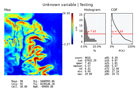
View map:

rs.view()

Convert and get an Univar instance:

uv = rs.get_univar()
print(type(uv))

<class 'plans.analyst.Univar'>

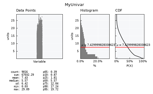
View as Univar:

uv.view()

Export to other file

Tif format is exported by default.

fo = rs.export(folder=OUTPUT_DIR, filename="slope_example")
print(fo)
print(f"File was created: {Path(fo).is_file()}")

outputs/raster/slope_example.tif
File was created: True

Copy raster structure

Sometimes it is useful to process raster data and then save it back to the same raster grid.

Example: making a brand new data grid with the same size using numpy.random

new_data = np.random.normal(loc=100, scale=10, size=np.shape(rs.data))
print(type(new_data))

<class 'numpy.ndarray'>

Define new raster, copy structure from other and set data:

# define a new raster
rs_new = Raster()
# copy structure from rs object
rs_new.copy_structure(raster_ref=rs)
# set data
rs_new.set_data(grid=new_data)

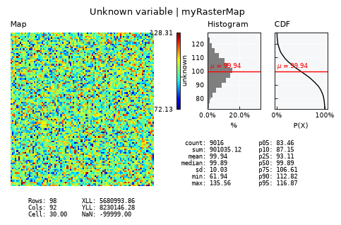
View and/or save

rs_new.view()

rs_new.export(folder=OUTPUT_DIR, filename="new_data")

'outputs/raster/new_data.tif'

Types of Rasters

The Raster class is extented into several families or types.

SciRaster family

This is a large family of rasters that are numerical values. Behaviour is nearly the same from Raster base class, but NODATA_value and dtype is enforced to the incoming data.

Members of this family are all conventional quantitative spatial variables, like terrain elevation or soil water content.

from plans.datasets import SciRaster

sciraster = SciRaster()
sciraster.load_data(file_data=raster_file)
print(f"Data type: {sciraster.dtype}")
print(f"No-data value: {sciraster.raster_metadata['NODATA_value']}")

Data type: float32
No-data value: -99999

View layout is the same from Raster:

sciraster.view()

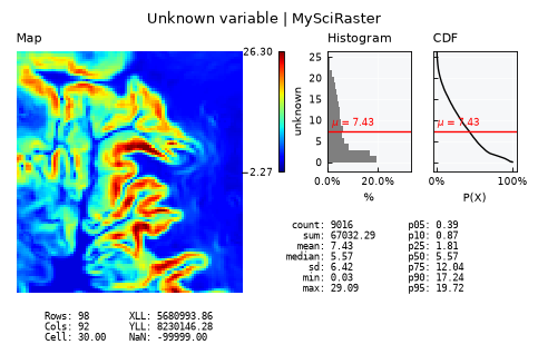
QualiRaster family

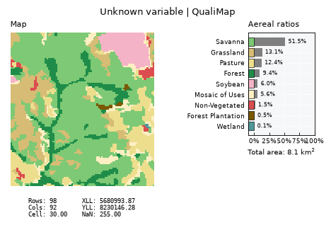
This is a large family of rasters that supports categorical maps, eg., land use maps. Data is always accompanied by an auxiliar Attribute Table with id, name, alias and color fields:

from plans.datasets import QualiRaster

Define new files (raster and table):

quali_raster_file = Path(pj.folder_lulc) / "observed/lulc_2020-01-01.tif"
quali_raster_table = Path(pj.folder_lulc) / "observed/lulc_attributes.csv"

qualiraster = QualiRaster()
qualiraster.load_data(
    file_data=quali_raster_file,
    file_table=quali_raster_table
)
print(f"Data type: {qualiraster.dtype}")
print(f"No-data value: {qualiraster.raster_metadata['NODATA_value']}")

Data type: uint8
No-data value: 255

Access the Attribute Table:

qualiraster.table.head()

	id	alias	name	name_pt	color	w_ck	w_ca	w_sk	w_soa	w_soc	w_sua	w_suc	w_sux	w_dea
0	3	Fr	Forest	Floresta	#1f8d49	10	1	1	1	1	1	1	1	1
1	4	Sv	Savanna	Savana	#7dc975	5	1	1	1	1	1	1	1	1
2	5	Mg	Mangrove	Mangue	#04381d	1	1	1	1	1	1	1	1	1
3	6	Fl	Floodable Forest	Floresta inundável	#026975	10	1	1	1	1	1	1	1	1
4	9	Fp	Forest Plantation	Silvicultura	#7a5900	1	1	1	1	1	1	1	1	1

Get areas table:

areas_df = qualiraster.get_areas()
areas_df

	id	name	alias	color	count	area_m2	area_ha	area_km2	area_f	area_%
0	3	Forest	Fr	#1f8d49	843	758700.0	75.87	0.7587	0.093500	9.350044
1	4	Savanna	Sv	#7dc975	4644	4179600.0	417.96	4.1796	0.515084	51.508429
2	5	Mangrove	Mg	#04381d	0	0.0	0.00	0.0000	0.000000	0.000000
3	6	Floodable Forest	Fl	#026975	0	0.0	0.00	0.0000	0.000000	0.000000
4	9	Forest Plantation	Fp	#7a5900	43	38700.0	3.87	0.0387	0.004769	0.476930
5	11	Wetland	We	#519799	6	5400.0	0.54	0.0054	0.000665	0.066548
6	12	Grassland	Gr	#d6bc74	1183	1064700.0	106.47	1.0647	0.131211	13.121118
7	13	Not-Forest	Nf	#d89f5c	0	0.0	0.00	0.0000	0.000000	0.000000
8	15	Pasture	Ps	#edde8e	1117	1005300.0	100.53	1.0053	0.123891	12.389086
9	20	Sugar cane	Sc	#db7093	0	0.0	0.00	0.0000	0.000000	0.000000
10	21	Mosaic of Uses	Mu	#ffefc3	505	454500.0	45.45	0.4545	0.056012	5.601154
11	23	Beach, Dune and Sand Spot	Sd	#ffa07a	0	0.0	0.00	0.0000	0.000000	0.000000
12	24	Urban Area	Ur	#d4271e	0	0.0	0.00	0.0000	0.000000	0.000000
13	25	Non-Vegetated	Nv	#db4d4f	137	123300.0	12.33	0.1233	0.015195	1.519521
14	29	Rocky Outcrop	Ro	#ffaa5f	0	0.0	0.00	0.0000	0.000000	0.000000
15	30	Mining	Mi	#9c0027	0	0.0	0.00	0.0000	0.000000	0.000000
16	31	Aquaculture	Aq	#091077	0	0.0	0.00	0.0000	0.000000	0.000000
17	32	Hypersaline Tidal Flat	Sf	#fc8114	0	0.0	0.00	0.0000	0.000000	0.000000
18	33	River, Lake and Ocean	W	#2532e4	0	0.0	0.00	0.0000	0.000000	0.000000
19	35	Palm Oil	Po	#9065d0	0	0.0	0.00	0.0000	0.000000	0.000000
20	39	Soybean	Sy	#f5b3c8	538	484200.0	48.42	0.4842	0.059672	5.967169
21	40	Rice	Rc	#c71585	0	0.0	0.00	0.0000	0.000000	0.000000
22	41	Temporary Crops	Tc	#f54ca9	0	0.0	0.00	0.0000	0.000000	0.000000
23	46	Coffee	Cf	#d68fe2	0	0.0	0.00	0.0000	0.000000	0.000000
24	47	Citrus	Ci	#9932cc	0	0.0	0.00	0.0000	0.000000	0.000000
25	48	Other Perennial Crops	Pc	#e6ccff	0	0.0	0.00	0.0000	0.000000	0.000000
26	49	Wooded Sandbank Vegetation	Ws	#02d659	0	0.0	0.00	0.0000	0.000000	0.000000
27	50	Herbaceous Sandbank Vegetation	Hs	#ad5100	0	0.0	0.00	0.0000	0.000000	0.000000
28	62	Cotton	Ct	#ff69b4	0	0.0	0.00	0.0000	0.000000	0.000000
29	101	Dirty Road	Rd	#D2CFC0	0	0.0	0.00	0.0000	0.000000	0.000000
30	102	Paved Road	Rs	#D4AD9B	0	0.0	0.00	0.0000	0.000000	0.000000
31	103	Railway	Rr	#B5A295	0	0.0	0.00	0.0000	0.000000	0.000000
32	255	Not Observed	No	#ffffff	0	0.0	0.00	0.0000	0.000000	0.000000

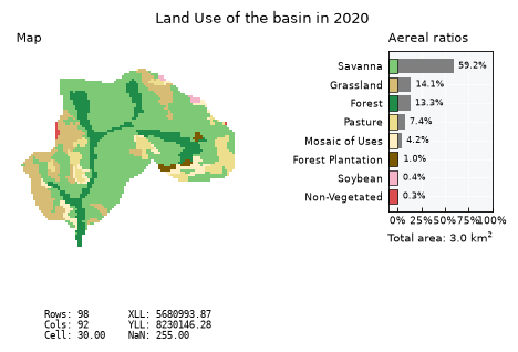
View scheme provides a horizontal bar for aereal ratios:

qualiraster.view()

Dedicated extensions

plans.datasets.spatial offers a series of dedicated Rasters for spatial variables. This helps to shortcut attributes and visual setup. Some examples are provided below.

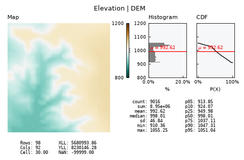
Elevation raster

from plans.datasets.spatial import Elevation
dem_file = Path(pj.folder_topo) / "dem.tif"
dem_raster = Elevation()
dem_raster.load_data(file_data=dem_file)
dem_raster.view_specs["range"] = [800, 1200]
dem_raster.view()

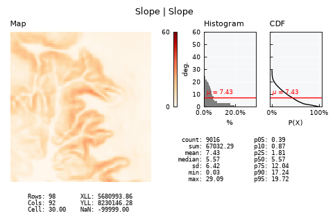
Slope raster

from plans.datasets.spatial import Slope
slope_file = Path(pj.folder_topo) / "slope.tif"
slope_raster = Slope()
slope_raster.load_data(file_data=slope_file)
slope_raster.view()

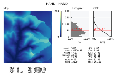
HAND raster

from plans.datasets.spatial import HAND
hand_file = Path(pj.folder_topo) / "hand.tif"
hand_raster = HAND()
hand_raster.load_data(file_data=hand_file)
hand_raster.view()

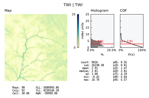
TWI raster

from plans.datasets.spatial import TWI
twi_file = Path(pj.folder_topo) / "twi.tif"
twi_raster = TWI()
twi_raster.load_data(file_data=twi_file)
twi_raster.view()

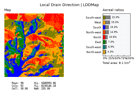
LDD raster

LDD (Local Drain Direction) is a core map for hydrological analysis. It depends on a convention of integer numbers.

from plans.datasets.spatial import LDD

ldd_file = Path(pj.folder_topo) / "ldd.tif"
ldd_raster = LDD()
ldd_raster.load_data(file_data=ldd_file)
ldd_raster.view()

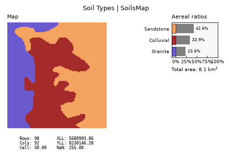
Soils raster

Soils may reflect soils classes and lithology. Requires the Attribute Table.

from plans.datasets.spatial import Soils
# define file
soils_file = Path(pj.folder_soils) / "soils.tif"
# define table
soils_table = Path(pj.folder_soils) / "soils_attributes.csv"
# define raster
soils_raster = Soils()
soils_raster.load_data(file_data=soils_file, file_table=soils_table)
soils_raster.view()

LULC raster

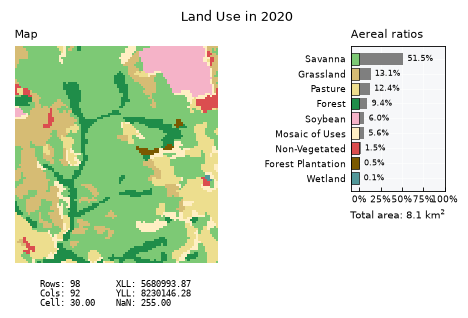
LULC (Land Use and Land Cover) requires the Attribute Table and date to be provided.

from plans.datasets.spatial import LULC
# define file
lulc_file = Path(pj.folder_lulc) / "observed/lulc_2020-01-01.tif"
# define table
lulc_table = Path(pj.folder_lulc) / "observed/lulc_attributes.csv"
# define name and datetime
lulc_raster = LULC(name="LULC", datetime="2020-01-01")
lulc_raster.load_data(file_data=lulc_file, file_table=lulc_table)
lulc_raster.view_specs["title"] = "Land Use in 2020"
lulc_raster.view()

AOI Raster

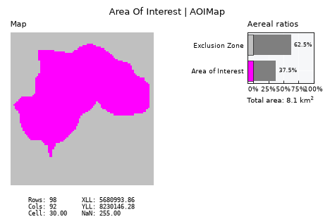
The AOI Raster (Area-Of-Interest) is a member of the QualiRaster family.

It is a boolean grid used mostly for masking operations. In this case, there is no need for an Attribute Table to be provided.

from plans.datasets import AOI
aoi = AOI()
# define basin raster for the AOI
aoi_file = Path(pj.folder_basins) / "main/basin.tif"
aoi.load_data(file_data=aoi_file)
aoi.view()

Masking Operations

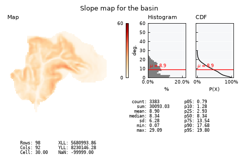
Masking is a very basic operation when working with Rasters, since in most cases we need to filter the data to a given AOI, like a catchment basin.

Say we want to know the average slope of a basin:

# use the data from the aoi map
slope_raster.apply_aoi_mask(grid_aoi=aoi.data)
slope_raster.view_specs["title"] = "Slope map for the basin"
slope_raster.view()

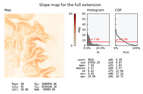
The AOI mask can be realeased:

slope_raster.release_aoi_mask()
slope_raster.view_specs["title"] = "Slope map for the full extension"
slope_raster.view()

The same can be done with qualitative maps:

lulc_raster.apply_aoi_mask(grid_aoi=aoi.data)
lulc_raster.view_specs["title"] = "Land Use of the basin in 2020"
lulc_raster.view()