Time Series - Seasonal ensembles

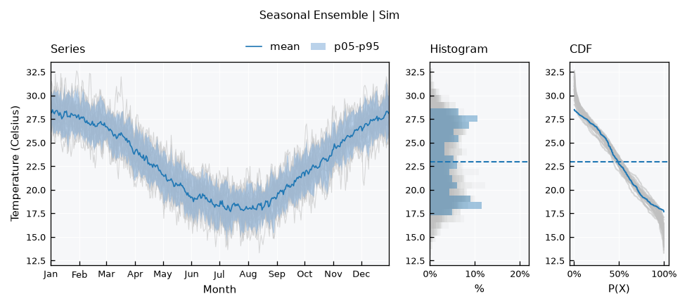
A SeasonalEnsemble treats the years of a single series as members of an ensemble. All years are drawn over the same calendar, which shows the seasonal cycle, how much it varies between years, and how one year compares with the others.

Covered here:

• Getting the ensemble from a series

• Highlighting a year

• Labels of the x axis

• Reducers and their dates

• Water years

• Monthly series and other time steps

See also

Check out the Time Series - Ensembles tutorial first. Reducers, bands and highlights work the same way here.

Notebook setup

For users running this tutorial as a Jupyter Notebook, this cell must be executed first:

import sys

# Install `plans` in `google.colab`.
# Use `pip install plans` for other environments.

if "google.colab" in sys.modules:
    import os
    os.system(f"{sys.executable} -m pip install -q plans")

from plans.datasets import RainSeries, TemperatureSeries

# This avoids warnings related to uninstalled fonts
import logging
logging.getLogger('matplotlib.font_manager').setLevel(logging.ERROR)

Get the ensemble from a series

Here is a synthetic daily temperature series of about 25 years, which stops in the middle of its last year. The .get_seasonal_ensemble() method splits it into one member per year, of the same type as the series. The series itself does not change:

ts = TemperatureSeries(name="Sim")
ts.generate(start="2000-01-01", end="2024-08-15", seed=1, inplace=True)

se = ts.get_seasonal_ensemble()
se.catalog[["name", "start", "end", "size"]].tail()

	name	start	end	size
20	2020	2000-01-01	2000-12-31	366
21	2021	2000-01-01	2000-12-31	365
22	2022	2000-01-01	2000-12-31	365
23	2023	2000-01-01	2000-12-31	365
24	2024	2000-01-01	2000-08-15	228

All members are on the same year, and 2000 is only a placeholder, chosen because it is a leap year. The incomplete year 2024 stays as a member and counts in the reducers where it has data.

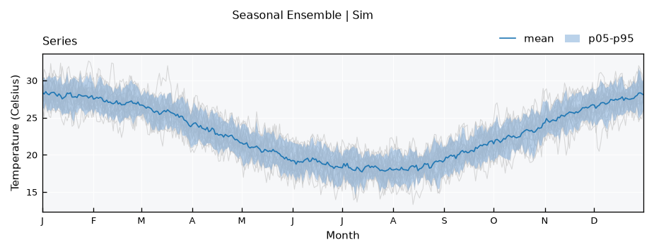
The default view draws the years in the background, with the mean and a percentile band on top:

se.view()

Highlight a year

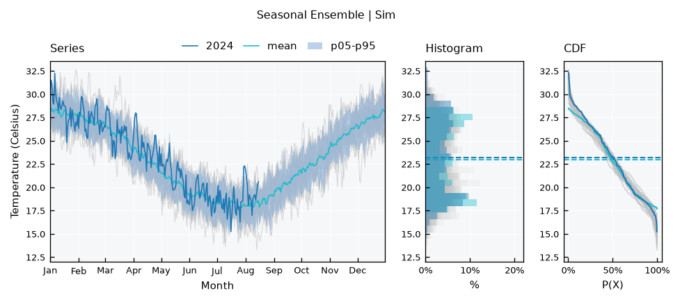
Members are named by year, as strings, so view_specs["highlight"] picks one out. This is how to compare the current year with the previous ones:

se.view_specs["highlight"] = ["2024"]
se.view()

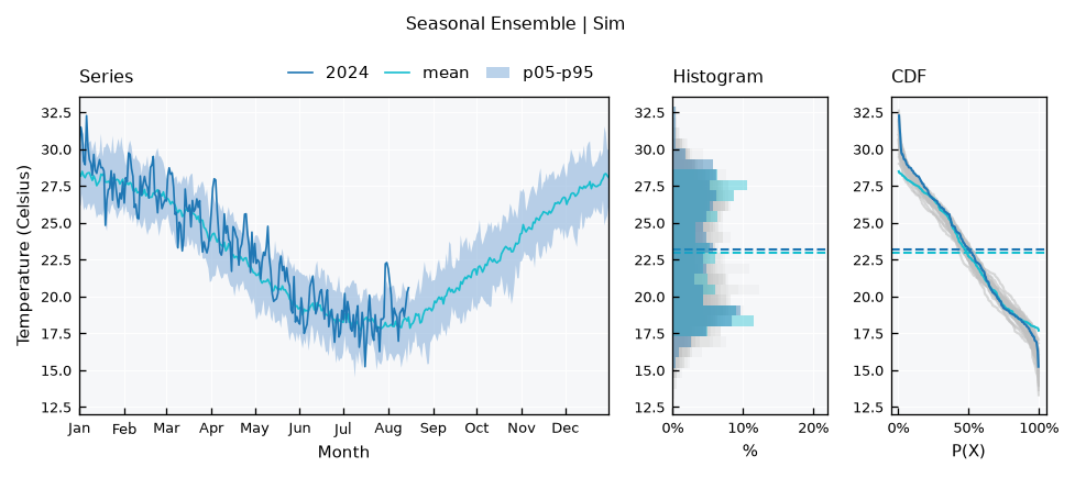
To see the year against the bands alone, hide the other years with view_specs["plot_background"]:

se.view_specs["plot_background"] = False
se.view()

Labels of the x axis

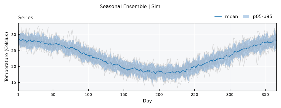
The xaxis spec sets the labels, and the options are month-alias (the default), month-letter, month and days. For instance, the day of the year, with the series-simple layout:

se.view_specs["highlight"] = None
se.view_specs["plot_background"] = True
se.view_specs["layout"] = "series-simple"
se.view_specs["xaxis"] = "days"
se.view()

Or the first letter of each month:

se.view_specs["xaxis"] = "month-letter"
se.view()

Note

The reference year is a leap year, so days always counts 29 Feb: 1 March is day 61, also for members that are not leap years.

Reducers and their dates

Reducers work across years at each step, as in a TimeSeriesEnsemble. They return a pandas.DataFrame with the datetime and one column per statistic, named {varalias}_{statistic}. The mean of each calendar day over all years:

se.mean().head()

	datetime	TAS_mean
0	2000-01-01	28.383279
1	2000-01-02	28.169339
2	2000-01-03	28.492458
3	2000-01-04	28.207311
4	2000-01-05	28.063112

Percentiles are named by their value:

se.percentiles(values=[5, 50, 95]).head()

	datetime	TAS_p05	TAS_p50	TAS_p95
0	2000-01-01	26.451995	28.479368	30.061823
1	2000-01-02	26.127887	28.137300	30.397375
2	2000-01-03	26.961585	28.590795	30.043051
3	2000-01-04	25.828472	28.212592	30.307475
4	2000-01-05	26.087131	28.083328	30.631371

And .stats() gives a combined table, with basic=True to keep only the quartiles:

se.stats(basic=True).head()

	datetime	TAS_sum	TAS_mean	TAS_std	TAS_min	TAS_max	TAS_p25	TAS_p50	TAS_p75
0	2000-01-01	709.581970	28.383279	1.069638	26.345397	30.182454	27.879470	28.479368	29.236899
1	2000-01-02	704.233486	28.169339	1.428355	25.111814	31.497556	27.255070	28.137300	28.902733
2	2000-01-03	712.311445	28.492458	1.139475	26.680771	31.003125	27.541150	28.590795	29.585939
3	2000-01-04	705.182779	28.207311	1.446431	25.684764	30.448555	27.031522	28.212592	29.382703
4	2000-01-05	701.577811	28.063112	1.471101	25.210212	30.984469	26.806353	28.083328	28.943544

The dates are on the reference year, so the row below is the average of all years on 5 March, and not a value from the year 2000:

df = se.mean()
df[df["datetime"] == "2000-03-05"]

	datetime	TAS_mean
64	2000-03-05	26.441786

To use these results with real dates, for instance to join them with the original series, use the month and day instead of the full date:

df["month_day"] = df["datetime"].dt.strftime("%m-%d")
df.head()

	datetime	TAS_mean	month_day
0	2000-01-01	28.383279	01-01
1	2000-01-02	28.169339	01-02
2	2000-01-03	28.492458	01-03
3	2000-01-04	28.207311	01-04
4	2000-01-05	28.063112	01-05

.get_reducer_series() returns a reducer as a series of the same type, also on the reference year:

ts_mean = se.get_reducer_series(name="mean")
print(type(ts_mean).__name__)
ts_mean.data.head()

TemperatureSeries

	datetime	tas
0	2000-01-01	28.383279
1	2000-01-02	28.169339
2	2000-01-03	28.492458
3	2000-01-04	28.207311
4	2000-01-05	28.063112

Note

Only leap years have a value on 29 Feb, so the reducers of that step use fewer members. With few leap years in the record, this can show as a one-day jump in the bands.

Water years

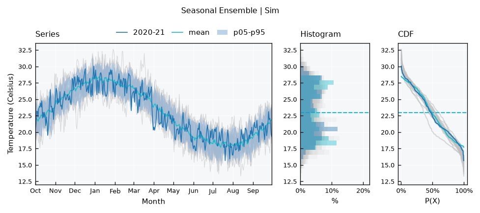
The year_start parameter sets the first month of the year. Members then hold two calendar years, and their names show both:

se_water = ts.get_seasonal_ensemble(year_start=10)
list(se_water.collection)[:3]

['1999-00', '2000-01', '2001-02']

The x axis starts on that month, and days counts from the start of the water year:

se_water.view_specs["highlight"] = ["2020-21"]
se_water.view()

Monthly series

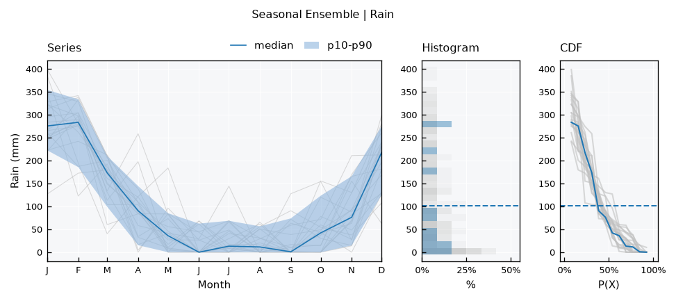
With monthly data this is the classical seasonal plot. Monthly dates are moved to the first day of the month, so it does not matter which day of the month the data use:

rain = RainSeries(name="Rain")
rain.generate(start="2000-01-01", end="2019-12-31", freq="MS", seed=1, inplace=True)

se_rain = rain.get_seasonal_ensemble()
se_rain.view_specs["reducers"] = ["median"]
se_rain.view_specs["bands"] = [[10, 90]]
se_rain.view_specs["xaxis"] = "month-letter"
se_rain.view()

Other time steps

The ensemble works with monthly, daily and shorter steps, because these steps fall on the same calendar positions every year. Other steps, like weekly data, do not, so each date would hold only a few members. These raise an error:

weekly = TemperatureSeries(name="Weekly")
weekly.generate(start="2000-01-01", end="2004-12-31", freq="7D", seed=1, inplace=True)

try:
    weekly.get_seasonal_ensemble()
except ValueError as e:
    print(e)

Time step of 7 days 00:00:00 does not repeat each year. Use a monthly, daily or shorter step

Recap

• .get_seasonal_ensemble() makes one member per year from a series, with incomplete years included.

• Reducers, bands, highlight and plot_background work as in a TimeSeriesEnsemble, and members are named by year.

• view_specs["xaxis"] sets the labels: month-alias, month-letter, month or days.

• Reducers return a pandas.DataFrame with one row per step of the year. Their dates, like those of the members, are placeholders of a leap reference year.

• year_start sets the first month, for water years.

• Time steps must repeat each year: monthly, daily or shorter.