
Databases - Basics#
This tutorial covers DataBase, the SQLite database of plans for time series of environmental variables. The example is a single weather station with monthly air temperature and rainfall.
See also
The database relies on three catalogs that ship with plans: variables, statistics and flags.
Notebook setup#
For users running this tutorial as a Jupyter Notebook, this cell must be executed first:
import sys
import json
from pathlib import Path
import numpy as np
import pandas as pd
import matplotlib.pyplot as plt

# Install `plans` in `google.colab`.
# Use `pip install plans` for other environments.

if "google.colab" in sys.modules:
    import os
    os.system(f"{sys.executable} -m pip install -q plans")

from plans.databases import DataBase

# This avoids warnings related to uninstalled fonts
import logging
# Set the matplotlib font manager logger to only show errors (hides warnings)
logging.getLogger('matplotlib.font_manager').setLevel(logging.ERROR)

# define output folder
OUTPUT_DIR = Path("outputs/databases")
OUTPUT_DIR.mkdir(parents=True, exist_ok=True)
print(f"Outputs will be saved to: ./{OUTPUT_DIR}")
Outputs will be saved to: ./outputs/databases
Describing the datasets#
A database stores records: one value at one time. Each record belongs to a spec, which describes a dataset: what variable it measures, which statistic summarizes each value over the time step, and where the data comes from. These three fields point to the catalogs by name.
Spec names are uppercase, with letters, digits and _. Here, a monthly mean temperature and a monthly rainfall total:
specs = [
    {
        "name": "TAS_MONTHLY",
        "abstract": "Monthly mean air temperature at the station (synthetic)",
        "method": "mean of daily readings",
        "timestep": "1M",
        "extent": "station",
        "scale": 1,
        "offset": 0,
        "start": "2001-01-01",
        "end": None,
        "variable_name": "surface air temperature",
        "statistic_name": "mean",
        "source_name": "INMET",
    },
    {
        "name": "PPT_MONTHLY",
        "abstract": "Monthly rainfall total at the station (synthetic)",
        "method": "sum of daily readings",
        "timestep": "1M",
        "extent": "station",
        "scale": 1,
        "offset": 0,
        "start": "2001-01-01",
        "end": None,
        "variable_name": "precipitation",
        "statistic_name": "sum",
        "source_name": "INMET",
    },
]
file_specs = OUTPUT_DIR / "station_specs.json"
file_specs.write_text(json.dumps(specs, indent=2), encoding="utf-8")
print(f"Specs saved to: ./{file_specs}")
Specs saved to: ./outputs/databases/station_specs.json
Creating the database#
The .new() method creates the file from a setup. The setup is a dict, or a TOML or JSON file with the same structure. It needs the path of the database and the path of the specs file. Catalogs come from plans unless the setup points to other files. With overwrite=True, an existing file is replaced, so this notebook can run again:
db = DataBase(name="Station")
file_db = db.new(
    config={
        "database": {"path": str(OUTPUT_DIR / "station.db")},
        "specs": {"path": str(file_specs)},
    },
    overwrite=True,
)
print(db.inspect_schema(quiet=True))
[Station]
  records  (0 rows)                   specs  (2 rows)                     flags  (10 rows)
    id                   INTEGER        id                   INTEGER        id                   INTEGER
    inserted             INTEGER        name                 TEXT           name                 TEXT
    datetime             INTEGER        abstract             TEXT           abstract             TEXT
    value                REAL           method               TEXT           alias                TEXT
    flag_value           INTEGER        timestep             TEXT           value                INTEGER
    spec_id              INTEGER        extent               TEXT
                                        scale                REAL
                                        offset               REAL
                                        start                INTEGER
                                        end                  INTEGER
                                        variable_name        TEXT
                                        statistic_name       TEXT
                                        source_name          TEXT

  variables  (153 rows)               statistics  (32 rows)               sources  (3 rows)
    id                   INTEGER        id                   INTEGER        id                   INTEGER
    code                 TEXT           name                 TEXT           name                 TEXT
    name                 TEXT           alias                TEXT           alias                TEXT
    alias                TEXT           title                TEXT           title                TEXT
    symbol               TEXT           abstract             TEXT           abstract             TEXT
    title                TEXT           symbol               TEXT           citation             TEXT
    abstract             TEXT           formula              TEXT           url                  TEXT
    synonyms             TEXT
    units                TEXT
    dimension            TEXT
    dtype                TEXT
    domain               TEXT
    discipline           TEXT
    theme                TEXT
    category             TEXT
    source               TEXT
    url                  TEXT
Larger projects often keep the setup in a file, and pass its path instead: db.new(config="station_setup.toml"). This setup, as a file:
[database]
path = "outputs/databases/station.db"

[specs]
path = "outputs/databases/station_specs.json"
{
  "database": {"path": "outputs/databases/station.db"},
  "specs": {"path": "outputs/databases/station_specs.json"}
}
Relative paths follow the working directory, not the setup file. Both formats refuse single backslashes, so Windows paths are written with forward slashes.
The database is now connected. The catalogs are plain tables, so SQL works on them. The units and the valid domain of each variable come from the variables table:
db.query_sql(
    sql="SELECT code, name, units, domain FROM variables WHERE name IN (?, ?)",
    params=["surface air temperature", "precipitation"],
)
| code | name | units | domain | |
|---|---|---|---|---|
| 0 | CLM100 | precipitation | mm/(dt) | [0U) |
| 1 | CLM001 | surface air temperature | degC | (U) |
print(db.inspect_specs(quiet=True))
[Station — specs]

  TAS_MONTHLY  (id 1)
       surface air temperature · mean · 1M · station
       source: INMET
       period: 2001-01-01 → open
       method: mean of daily readings
       Monthly mean air temperature at the station (synthetic)

  PPT_MONTHLY  (id 2)
       precipitation · sum · 1M · station
       source: INMET
       period: 2001-01-01 → open
       method: sum of daily readings
       Monthly rainfall total at the station (synthetic)
Sample data#
Lets make 20 years of monthly data. Temperature follows a seasonal cycle, warmer in January, as in the southern hemisphere. Rainfall is drawn from a gamma distribution whose mean also changes with the season:
rng = np.random.default_rng(seed=42)  # ensure reproducibility

dates = pd.date_range(start="2001-01-01", end="2020-12-01", freq="MS")
season = np.cos(2 * np.pi * (dates.month - 1) / 12)

df_tas = pd.DataFrame(
    {"datetime": dates, "value": 19 + 5 * season + rng.normal(scale=1, size=len(dates))}
)
mean_ppt = 120 - 30 * season
df_ppt = pd.DataFrame(
    {"datetime": dates, "value": rng.gamma(shape=4, scale=mean_ppt / 4)}
)
df_ppt.head()
| datetime | value | |
|---|---|---|
| 0 | 2001-01-01 | 50.194364 |
| 1 | 2001-02-01 | 28.809903 |
| 2 | 2001-03-01 | 247.847522 |
| 3 | 2001-04-01 | 58.258278 |
| 4 | 2001-05-01 | 422.441777 |
Real data is never this clean. Lets add two problems to the rainfall: a month the station did not report, and a negative value from a faulty sensor:
df_ppt.loc[30, "value"] = np.nan
df_ppt.loc[90, "value"] = -12.0
df_ppt.loc[[30, 90]]
| datetime | value | |
|---|---|---|
| 30 | 2003-07-01 | NaN |
| 90 | 2008-07-01 | -12.0 |
Inserting records#
The .insert_records() method takes a DataFrame with datetime and value columns, the spec name, and a flag for the batch. Flag 1 is regular. Dates can be text or datetimes; they are stored as epoch seconds:
db.insert_records(dataframe=df_tas, spec_name="TAS_MONTHLY", flag=1)
For the rainfall, two things happen. Missing values are dropped by default; with nan_policy="void", they are stored as an empty value with the void flag (0), so the gap reported by the station is kept. And values outside the domain of the variable, [0U) for precipitation, turn from regular into suspect (2), with a warning. The value is kept for review:
import warnings

# catch the warning here only to print its message
with warnings.catch_warnings(record=True) as caught:
    warnings.simplefilter("always")
    db.insert_records(dataframe=df_ppt, spec_name="PPT_MONTHLY", flag=1, nan_policy="void")
for warning in caught:
    print(f"{warning.category.__name__}: {warning.message}")
UserWarning: 1 value(s) of PPT_MONTHLY outside [0U) flagged suspect
print(db.inspect_records(head=5, quiet=True))
[Station]
  records  (480 rows)
    id                   INTEGER
    inserted             INTEGER
    datetime             INTEGER
    value                REAL
    flag_value           INTEGER
    spec_id              INTEGER

  head (5)
 id         inserted         datetime     value  flag_value  spec_id
  1 2026-11-09 18:55 2001-01-01 00:00 24.304717           1        1
  2 2026-11-09 18:55 2001-02-01 00:00 22.290143           1        1
  3 2026-11-09 18:55 2001-03-01 00:00 22.250451           1        1
  4 2026-11-09 18:55 2001-04-01 00:00 19.940565           1        1
  5 2026-11-09 18:55 2001-05-01 00:00 14.548965           1        1
Querying records#
The .query_records() method takes all filters and options in one dict. By default, it returns the long format, one row per record, with datetime as a UTC timestamp:
df = db.query_records(
    query_dict={"spec_name": "PPT_MONTHLY", "start": "2003-01-01", "end": "2003-12-31"}
)
df[["datetime", "value", "flag_value", "spec_name"]]
| datetime | value | flag_value | spec_name | |
|---|---|---|---|---|
| 0 | 2003-01-01 00:00:00+00:00 | 94.391632 | 1 | PPT_MONTHLY |
| 1 | 2003-02-01 00:00:00+00:00 | 73.691661 | 1 | PPT_MONTHLY |
| 2 | 2003-03-01 00:00:00+00:00 | 84.131814 | 1 | PPT_MONTHLY |
| 3 | 2003-04-01 00:00:00+00:00 | 218.032488 | 1 | PPT_MONTHLY |
| 4 | 2003-05-01 00:00:00+00:00 | 109.065666 | 1 | PPT_MONTHLY |
| 5 | 2003-06-01 00:00:00+00:00 | 155.584754 | 1 | PPT_MONTHLY |
| 6 | 2003-07-01 00:00:00+00:00 | NaN | 0 | PPT_MONTHLY |
| 7 | 2003-08-01 00:00:00+00:00 | 294.463555 | 1 | PPT_MONTHLY |
| 8 | 2003-09-01 00:00:00+00:00 | 188.391552 | 1 | PPT_MONTHLY |
| 9 | 2003-10-01 00:00:00+00:00 | 106.514657 | 1 | PPT_MONTHLY |
| 10 | 2003-11-01 00:00:00+00:00 | 80.398374 | 1 | PPT_MONTHLY |
| 11 | 2003-12-01 00:00:00+00:00 | 115.158401 | 1 | PPT_MONTHLY |
Flags select records. Here, the records that need attention:
df = db.query_records(query_dict={"flag_value": [0, 2]})
df[["datetime", "value", "flag_value", "spec_name"]]
| datetime | value | flag_value | spec_name | |
|---|---|---|---|---|
| 0 | 2003-07-01 00:00:00+00:00 | NaN | 0 | PPT_MONTHLY |
| 1 | 2008-07-01 00:00:00+00:00 | -12.0 | 2 | PPT_MONTHLY |
The wide format has one column per spec, indexed by datetime. With with_meta, the variable, units, statistic and source of each spec go to .attrs["specs"]. Selecting only regular records leaves the gap and the suspect month empty:
wide = db.query_records(
    query_dict={
        "spec_name": ["TAS_MONTHLY", "PPT_MONTHLY"],
        "flag_value": 1,
        "wide": True,
        "with_meta": True,
    }
)
wide.head()
| spec_name | TAS_MONTHLY | PPT_MONTHLY |
|---|---|---|
| datetime | ||
| 2001-01-01 00:00:00+00:00 | 24.304717 | 50.194364 |
| 2001-02-01 00:00:00+00:00 | 22.290143 | 28.809903 |
| 2001-03-01 00:00:00+00:00 | 22.250451 | 247.847522 |
| 2001-04-01 00:00:00+00:00 | 19.940565 | 58.258278 |
| 2001-05-01 00:00:00+00:00 | 14.548965 | 422.441777 |
meta = wide.attrs["specs"].set_index("spec_name")
meta
| variable_name | units | statistic_name | source_name | |
|---|---|---|---|---|
| spec_name | ||||
| TAS_MONTHLY | surface air temperature | degC | mean | INMET |
| PPT_MONTHLY | precipitation | mm/(dt) | sum | INMET |
fig, axes = plt.subplots(nrows=2, ncols=1, figsize=(8, 5), sharex=True)
axes[0].plot(wide.index, wide["TAS_MONTHLY"], color="tab:red", lw=1)
axes[0].set_ylabel(f'Temperature ({meta.loc["TAS_MONTHLY", "units"]})')
axes[1].bar(wide.index, wide["PPT_MONTHLY"], width=25, color="tab:blue")
axes[1].set_ylabel(f'Rainfall ({meta.loc["PPT_MONTHLY", "units"]})')
plt.tight_layout()
plt.show()
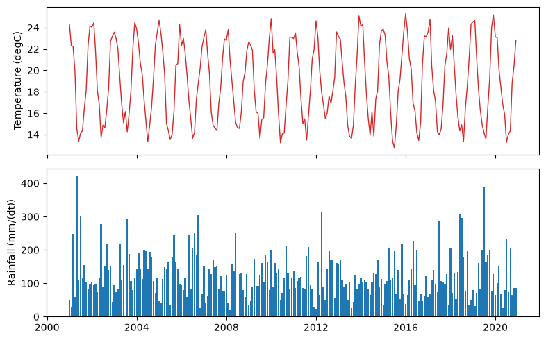
As a DataFrame, the result goes straight into pandas. The mean year:
wide.groupby(wide.index.month).mean().round(1)
| spec_name | TAS_MONTHLY | PPT_MONTHLY |
|---|---|---|
| datetime | ||
| 1 | 23.7 | 98.1 |
| 2 | 23.3 | 84.3 |
| 3 | 21.2 | 110.6 |
| 4 | 19.0 | 133.7 |
| 5 | 16.4 | 140.4 |
| 6 | 14.7 | 133.7 |
| 7 | 14.4 | 175.6 |
| 8 | 14.4 | 145.6 |
| 9 | 16.3 | 151.2 |
| 10 | 18.9 | 133.1 |
| 11 | 21.6 | 92.7 |
| 12 | 23.5 | 91.4 |
Closing and reopening#
The .close() method releases the file. Later, .connect() opens it again, with all the records in place:
db.close()

db = DataBase(name="Station")
db.connect(file_db=file_db)
print(len(db.query_records()), "records")
db.close()
480 records