Time Series - Collection visuals

A collection can answer different questions, and each question has its own picture. Is there data, and when? How do different variables relate over time? Do several sites or model runs agree? This tutorial goes through the visuals of the time series collections from those questions, using a small synthetic catchment.

All visuals follow the same pattern: choose a layout in view_specs, adjust other specs if needed, and call .view().

Covered here:

• Choosing a visual for each question

• Data availability: the full and simple layouts

• Stacked panels: the stacked and stacked-simple layouts

• Specs of the collection and specs of each series

• Common uses: rain, streamflow and storage; model and error; series decomposition

• Comparing series of the same variable: clusters and ensembles

• Saving a figure and adding to it

See also

Check out the Time Series - Collections tutorial for how collections work.

Which visual?

Question	Object	Layout
When is there data, and where do records overlap?	any collection	full, simple
How do different variables behave over the same time?	any collection	stacked, stacked-simple
Do sites of the same variable agree?	TimeSeriesCluster	series, series-simple
How similar are the sites, as numbers?	TimeSeriesCluster	correlation
What is the spread of many realizations?	TimeSeriesEnsemble	series, series-simple
How does the year vary, and how does this year compare?	SeasonalEnsemble	series, series-simple

The -simple layouts leave out the histograms and CDFs, which gives the time axis the full width of the figure.

Notebook setup

For users running this tutorial as a Jupyter Notebook, this cell must be executed first:

import sys
import numpy as np
import pandas as pd

# Install `plans` in `google.colab`.
# Use `pip install plans` for other environments.

if "google.colab" in sys.modules:
    import os
    os.system(f"{sys.executable} -m pip install -q plans")

from plans.datasets import (
    ETSeries,
    PETSeries,
    RainSeries,
    StreamflowSeries,
    TemperatureSeries,
    TimeSeries,
    TimeSeriesCluster,
    TimeSeriesCollection,
)

# This avoids warnings related to uninstalled fonts
import logging
logging.getLogger('matplotlib.font_manager').setLevel(logging.ERROR)

rng = np.random.default_rng(seed=7)  # ensure reproducibility

A synthetic catchment

Rain and potential evapotranspiration come from the generators of each series. A simple water balance turns them into evapotranspiration, streamflow and storage: the catchment is a single reservoir, which loses water in proportion to how much it holds. The observed streamflow is the simulated one with some measurement error, and two measurement gaps.

start, end = "2018-01-01", "2021-12-31"
df_rain = RainSeries(name="Rain").generate(start=start, end=end, seed=1)
df_pet = PETSeries(name="PET").generate(start=start, end=end, seed=2)

# water balance of a single reservoir
n = len(df_rain)
vct_et, vct_q, vct_s = np.zeros(n), np.zeros(n), np.zeros(n)
storage = 100.0
for i in range(n):
    vct_et[i] = df_pet["pet"].values[i] * min(1, storage / 150)
    vct_q[i] = 0.05 * storage
    storage = max(0, storage + df_rain["ppt"].values[i] - vct_et[i] - vct_q[i])
    vct_s[i] = storage

df = pd.DataFrame(
    {
        "datetime": df_rain["datetime"],
        "Rain": df_rain["ppt"],
        "PET": df_pet["pet"],
        "ET": vct_et,
        "Simulated": vct_q,
        "Observed": vct_q * rng.lognormal(mean=0, sigma=0.15, size=n),
        "Storage": vct_s,
    }
)

# measurement gaps
df.loc[df["datetime"].between("2019-04-01", "2019-08-15"), "Observed"] = np.nan
df.loc[df["datetime"].between("2020-11-01", "2020-12-10"), "Observed"] = np.nan
df["Error"] = df["Simulated"] - df["Observed"]
df.head()

	datetime	Rain	PET	ET	Simulated	Observed	Storage	Error
0	2018-01-01	10.285795	5.558449	3.705633	5.000000	5.000923	101.580162	-0.000923
1	2018-01-02	11.431808	5.318397	3.601624	5.079008	5.311784	104.331337	-0.232776
2	2018-01-03	10.970837	5.217987	3.629331	5.216567	5.006409	106.456276	0.210158
3	2018-01-04	7.791624	4.352178	3.088778	5.322814	4.657195	105.836309	0.665619
4	2018-01-05	10.755277	5.514332	3.890777	5.291815	4.942942	107.408994	0.348873

Each column goes into a series of its own class, which brings the variable name and the units. Gaps stay as empty rows, so lines break there. With dropnan=True, these rows are dropped and a line goes straight across a gap, until .standardize() brings them back. There is no class for storage or errors, so these two are plain TimeSeries. The temperature is independent of the rest, and starts a year later, so the next section has something to show.

Note that .append() stores a copy of the series. To change a series afterwards, reach it through tsc.collection[name].

def make_series(name, cls=TimeSeries, varname=None):
    ts = cls(name=name, alias=name[:3])
    if varname is not None:
        ts.varname = varname
        ts.units = "mm"
    ts.set_data(input_df=df, input_dtfield="datetime", input_varfield=name)
    return ts

tsc = TimeSeriesCollection(name="Catchment")
for ts in [
    make_series(name="Rain", cls=RainSeries),
    make_series(name="PET", cls=PETSeries),
    make_series(name="ET", cls=ETSeries),
    make_series(name="Simulated", cls=StreamflowSeries),
    make_series(name="Observed", cls=StreamflowSeries),
    make_series(name="Error", varname="Error"),
    make_series(name="Storage", varname="Storage"),
]:
    tsc.append(new_object=ts)

# a shorter record
ts_tas = TemperatureSeries(name="Temperature", alias="Tem")
ts_tas.generate(start="2019-01-01", end=end, seed=3, inplace=True)
tsc.append(new_object=ts_tas)

tsc.update(details=True)
tsc.catalog[["name", "alias", "units", "start", "end"]]

	name	alias	units	start	end
0	ET	ET	mm	2018-01-01	2021-12-31
1	Error	Err	mm	2018-01-01	2021-12-31
2	Observed	Obs	mm	2018-01-01	2021-12-31
3	PET	PET	mm	2018-01-01	2021-12-31
4	Rain	Rai	mm	2018-01-01	2021-12-31
5	Simulated	Sim	mm	2018-01-01	2021-12-31
6	Storage	Sto	mm	2018-01-01	2021-12-31
7	Temperature	Tem	Celsius	2019-01-01	2021-12-31

When is there data?

The default full layout does not draw any values. It is a map of the records, usually the first thing to check in a new dataset. The Gantt chart (a) has a bar for each continuous stretch of each series, so gaps show as breaks. The overlap (b) gives the share of series with data at each time, and the prevalence (c) gives the share of the whole period that each series covers.

tsc.view()

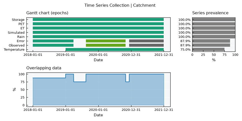
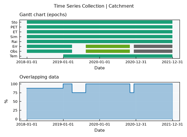
The observed streamflow shows its two gaps, and the temperature starts late. The drop in the overlap marks the periods where any analysis combining these series loses data. The simple layout leaves out the prevalence, and usealias swaps names for aliases, which helps with long names:

tsc.view_specs["layout"] = "simple"
tsc.view_specs["usealias"] = True
tsc.view()
tsc.view_specs["usealias"] = False

Stacked panels

The stacked layout draws one panel per row with a common time axis, so events line up from top to bottom. Each row has the series, its histogram and its CDF, just like the view of a single series.

The panels spec tells which series go where, as a list with the names of each panel. Here is the classic reading of a catchment, where rain drives storage and storage drives streamflow:

tsc.view_specs["layout"] = "stacked"
tsc.view_specs["panels"] = [["Rain"], ["Storage"], ["Simulated"]]
tsc.view()

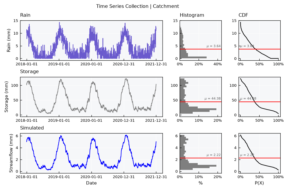
With panels set to None, which is the default, each series of the collection gets its own panel, in the order of the catalog. The height of the figure follows the number of panels, so this gets tall quickly.

Several series on a panel

A panel takes any number of series. Their histograms and CDFs are overlaid, using common bins so they can be compared, and the mean lines become dashed. A legend appears at the top of the panel. Each series uses its own color, so here the observed streamflow goes in black to stand out from the simulated one:

tsc.collection["Observed"].view_specs["color"] = "black"

tsc.view_specs["panels"] = [["Rain"], ["PET", "ET"], ["Observed", "Simulated"]]
tsc.view()

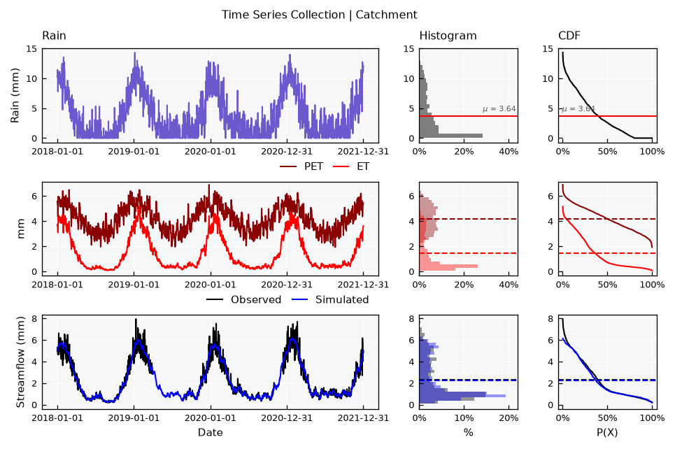
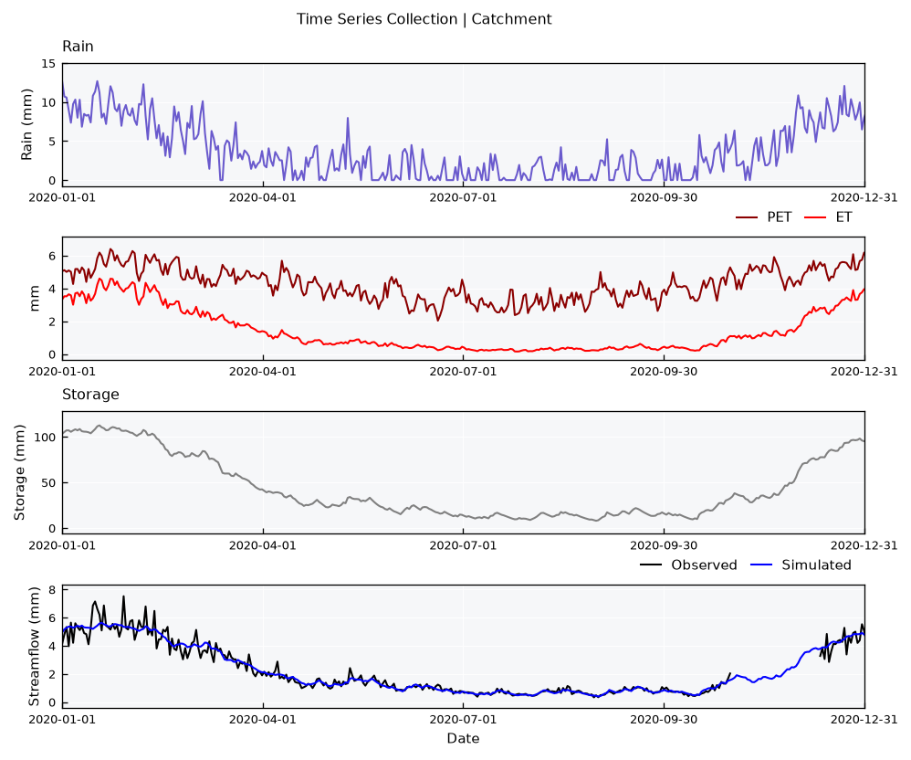
ET follows PET when the reservoir is full and falls behind it when the reservoir runs low, which is hard to see in separate panels. The gaps of the observed series simply show as breaks in the line.

Series in a panel share one y axis, so they must have the same units. A mix raises an error rather than producing a misleading figure:

tsc.view_specs["panels"] = [["Rain", "Temperature"]]
try:
    tsc.view()
except ValueError as e:
    print(e)

Series of a panel must have the same units. Got {'Rain': 'mm', 'Temperature': 'Celsius'}

Heights of the panels

Panels have equal heights by default. The panel_heights spec sets relative heights, which helps when one panel is the main subject. A model and its error is the typical case:

tsc.view_specs["panels"] = [["Observed", "Simulated"], ["Error"]]
tsc.view_specs["panel_heights"] = [3, 1]
tsc.view()

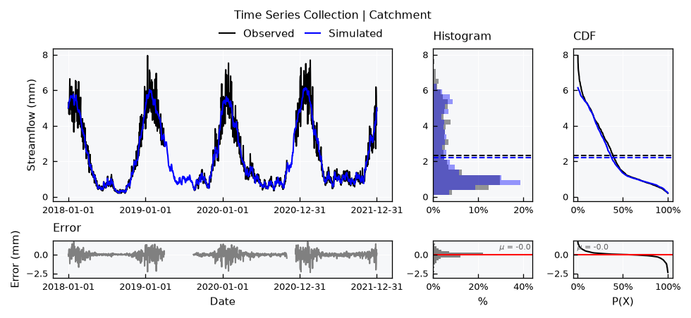
This spec stays in view_specs, like all others. It must have one value per panel, so remember to reset it when changing the panels.

Series only

The stacked-simple layout leaves out the histograms and CDFs. It suits long records and many panels, where the width helps more than the distributions do. The xmin and xmax specs zoom into a period:

tsc.view_specs["layout"] = "stacked-simple"
tsc.view_specs["panel_heights"] = None
tsc.view_specs["panels"] = [["Rain"], ["PET", "ET"], ["Storage"], ["Observed", "Simulated"]]
tsc.view_specs["xmin"] = pd.Timestamp("2020-01-01")
tsc.view_specs["xmax"] = pd.Timestamp("2020-12-31")
tsc.view()

Note

The xmin and xmax specs only change the time axis. In the stacked layout, histograms, CDFs and the y axis still describe the whole record. To get those for a period, filter the data of the series first.

Two levels of specs

A stacked figure takes specs from two places. The collection decides the figure, and each series decides its own look, in its own view_specs.

Where	Spec	What it does
Collection	layout, panels, panel_heights	The structure of the figure
Collection	title, xlabel, subtitle_hist, subtitle_cdf	Texts
Collection	xmin, xmax	The period
Collection	usealias	Aliases instead of names, in titles and legends
Collection	bins, alpha_hist, histtype, plot_mean	Histograms and means of shared panels
Collection	cmap_series	Where a replacement color comes from
Series	color, linewidth, alpha	The line
Series	fill, fill_only, color_fill	The area below the line
Series	color_hist, color_cdf, color_mean, bins	Histogram, CDF and mean of a lone series
Series	range	The y range. A shared panel covers the ranges of all its series

Here is rain as a filled area, in a fixed range, next to a streamflow in blue:

ts_rain = tsc.collection["Rain"]
ts_rain.view_specs["color"] = "tab:blue"
ts_rain.view_specs["color_hist"] = "tab:blue"
ts_rain.view_specs["color_cdf"] = "tab:blue"
ts_rain.view_specs["fill"] = True
ts_rain.view_specs["fill_only"] = True
ts_rain.view_specs["range"] = [0, 20]

ts_flow = tsc.collection["Simulated"]
ts_flow.view_specs["color"] = "navy"
ts_flow.view_specs["color_hist"] = "navy"
ts_flow.view_specs["color_cdf"] = "navy"

tsc.view_specs["layout"] = "stacked"
tsc.view_specs["xmin"] = None
tsc.view_specs["xmax"] = None
tsc.view_specs["panels"] = [["Rain"], ["Simulated"]]
tsc.view()

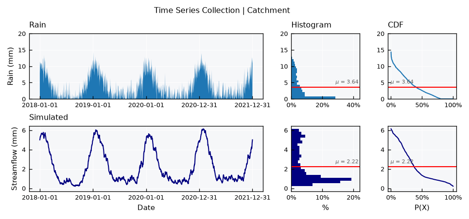
A shared panel uses the color of each series for the line, histogram, CDF and mean together. If two series of a panel have the same color, as the ones of the same class do by default, the repeated one takes the color of cmap_series farthest from those in use.

Series decomposition

The panels do not need to come from different sensors. A decomposition splits one series into parts that add up to it, and stacked panels read naturally for that. Here it is for twenty years of temperature with a warming trend. The trend comes from a centered moving average, the cycle from the average of each day of the year, and the remainder from what is left:

ts_warm = TemperatureSeries(name="Warming")
ts_warm.generator_specs["change_per_year"] = 0.1
df_t = ts_warm.generate(start="2000-01-01", end="2019-12-31", seed=4)

df_t["Trend"] = df_t["tas"].rolling(window=365, center=True).mean()
vct_doy = df_t["datetime"].dt.dayofyear
df_t["Cycle"] = (df_t["tas"] - df_t["Trend"]).groupby(vct_doy).transform("mean")
df_t["Remainder"] = df_t["tas"] - df_t["Trend"] - df_t["Cycle"]
df_t["Series"] = df_t["tas"]

tsc_parts = TimeSeriesCollection(name="Temperature decomposition")
for name in ["Series", "Trend", "Cycle", "Remainder"]:
    ts = TimeSeries(name=name, alias=name)
    ts.varname = "Temperature"
    ts.units = "C"
    ts.set_data(input_df=df_t, input_dtfield="datetime", input_varfield=name)
    tsc_parts.append(new_object=ts)
tsc_parts.update(details=True)

tsc_parts.view_specs["layout"] = "stacked"
tsc_parts.view_specs["panels"] = [["Series"], ["Trend"], ["Cycle"], ["Remainder"]]
tsc_parts.view()

/tmp/ipykernel_3144/2510135370.py:6: Pandas4Warning: Series.dt.dayofyear is deprecated and will be removed in a future version. Use Series.dt.day_of_year instead.
  vct_doy = df_t["datetime"].dt.dayofyear

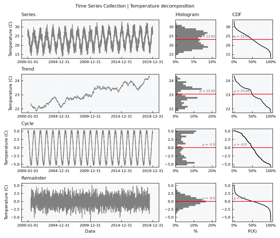
The catalog sorts the names alphabetically, so the panels spec is also how to set the reading order. Note how each panel keeps its own y range: the trend is much smaller than the cycle, but both fill their panels. Read the values on the axes before comparing the size of the parts. The trend and the remainder are also shorter than the series, as the moving average needs a full window on both sides.

Series of the same variable

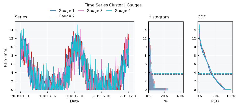
Some collections hold one variable only, and their series can share a single axis. The TimeSeriesCluster is for different sites, and adds the series, series-simple and correlation layouts. Here is a small network of rain gauges:

tsc_gauges = TimeSeriesCluster(name="Gauges", base_object=RainSeries)
for i in range(4):
    name = f"Gauge {i + 1}"
    ts = RainSeries(name=name, alias=f"G{i + 1}")
    ts.generate(start=start, end="2019-12-31", seed=10 + i, inplace=True)
    tsc_gauges.append(new_object=ts)
tsc_gauges.update(details=True)

tsc_gauges.view_specs["layout"] = "series"
tsc_gauges.view()

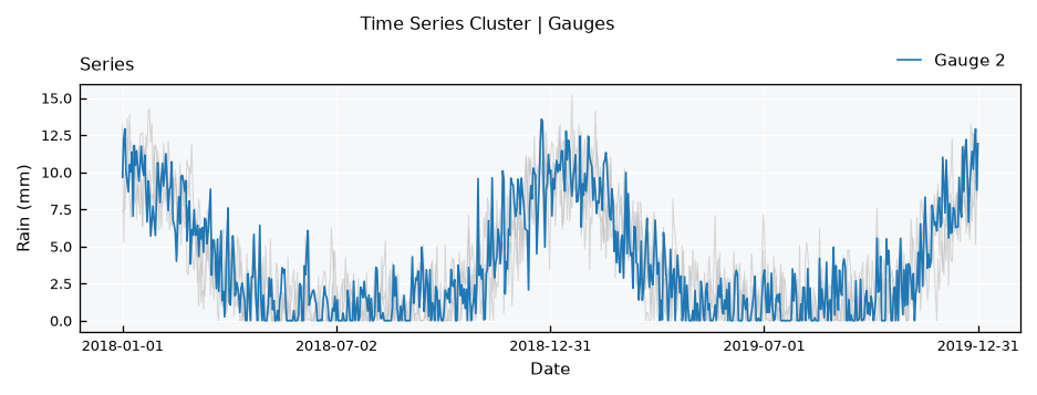
With many series, the highlight spec keeps a few in color and sends the others to the background:

tsc_gauges.view_specs["layout"] = "series-simple"
tsc_gauges.view_specs["highlight"] = ["Gauge 2"]
tsc_gauges.view()

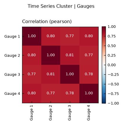
The correlation layout gives the same comparison as numbers. The weather of these gauges is independent, and they only share the cycle, which is already enough for high values:

tsc_gauges.view_specs["layout"] = "correlation"
tsc_gauges.view()

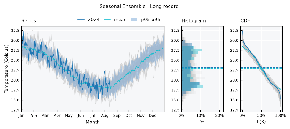
A TimeSeriesEnsemble is for many realizations of one series, like model runs. Its series layout draws the members in the background, with percentile bands and statistics on top. A SeasonalEnsemble does the same with the years of a single series, and it comes straight from the series:

ts_long = TemperatureSeries(name="Long record")
ts_long.generate(start="2000-01-01", end="2024-08-15", seed=1, inplace=True)

se = ts_long.get_seasonal_ensemble()
se.view_specs["highlight"] = ["2024"]
se.view()

See also

These objects have their own tutorials: Time Series - Clusters, Time Series - Ensembles and Time Series - Seasonal ensembles.

Saving a figure and adding to it

With show=False, the .view() method saves the figure instead of showing it. The file is {folder}/{filename}.{fig_format}, from the specs of the same names, and the folder must exist:

tsc.view_specs["folder"] = "./outputs"
tsc.view_specs["filename"] = "catchment"
tsc.view_specs["fig_format"] = "png"
tsc.view(show=False)

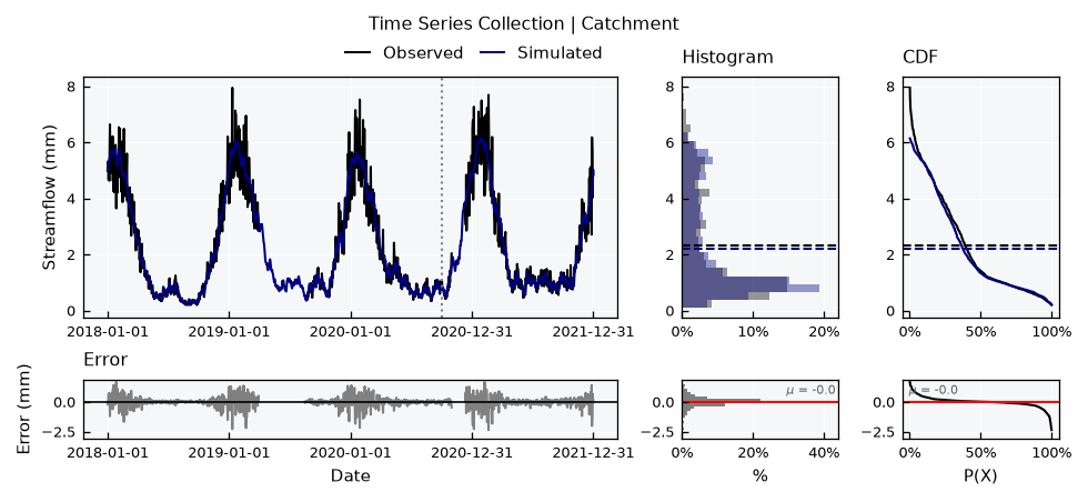
With return_fig=True, it returns the matplotlib figure, for adding things that the specs do not cover. The axes come panel by panel, and each panel of the stacked layout has three: series, histogram and CDF. Here is the zero line of the error, and a mark on a date of interest:

tsc.view_specs["panels"] = [["Observed", "Simulated"], ["Error"]]
tsc.view_specs["panel_heights"] = [3, 1]
fig = tsc.view(return_fig=True)

ax_flow, ax_error = fig.get_axes()[0], fig.get_axes()[3]
ax_error.axhline(y=0, color="black", linewidth=0.8)
ax_flow.axvline(x=pd.Timestamp("2020-10-01"), color="gray", linestyle="dotted");

Recap

• The layout spec chooses the visual, and the class decides which layouts are available. An unknown layout raises an error that lists the options.

• full and simple show when there is data, and stacked and stacked-simple show the values on a common time axis.

• panels sets which series go in each panel, panel_heights sets their relative sizes, and series in a panel must have the same units.

• The collection specs decide the figure, and the specs of each series decide its look.

• Clusters and ensembles add the series layouts, where series of one variable share an axis.

• return_fig=True gives the matplotlib figure, for anything else.