Time Series - Ensembles

A TimeSeriesEnsemble holds many realizations of the same series: the same variable, at the same site, over the same time. Typical examples are model runs with perturbed inputs or parameters, or draws of a stochastic generator. Unlike a TimeSeriesCluster, where each series is a different site, the members of an ensemble are interchangeable: what matters is how they spread at each time step.

Covered here:

• Assembling an ensemble

• Reducers: statistics across members at each time step

• Custom reducers

• Visuals, with reducers and percentile bands highlighted over the members

See also

Check out the Time Series - Clusters tutorial first.

Notebook setup

For users running this tutorial as a Jupyter Notebook, this cell must be executed first:

import sys
from pathlib import Path
import numpy as np
import pandas as pd

# Install `plans` in `google.colab`.
# Use `pip install plans` for other environments.

if "google.colab" in sys.modules:
    import os
    os.system(f"{sys.executable} -m pip install -q plans")

from plans.datasets import TemperatureSeries, TimeSeriesEnsemble

# This avoids warnings related to uninstalled fonts
import logging
logging.getLogger('matplotlib.font_manager').setLevel(logging.ERROR)

rng = np.random.default_rng(seed=5)  # ensure reproducibility

Build a synthetic ensemble

Fifty members of daily temperature over one year. Each member shares the cycle, but has its own bias and its own weather (an autoregressive anomaly), like runs of a model with uncertain inputs. Members are assembled in memory with .set_data() and .append():

n_members = 50
n = 365
t = np.arange(n)
dates = pd.date_range(start="2021-01-01", periods=n, freq="D")
cycle = 18 + 5 * np.sin(2 * np.pi * (t - 100) / 365)

def make_anomaly(phi, sd):
    # autoregressive anomaly: a[t] = phi * a[t-1] + shock
    a = np.zeros(n)
    e = rng.normal(loc=0, scale=sd, size=n)
    for i in range(1, n):
        a[i] = phi * a[i - 1] + e[i]
    return a

tse = TimeSeriesEnsemble(name="Projections", base_object=TemperatureSeries)
for k in range(n_members):
    bias = rng.normal(loc=0, scale=0.8)
    values = cycle + bias + make_anomaly(phi=0.85, sd=1.2)
    name = f"R{k + 1:02d}"
    ts = TemperatureSeries(name=name, alias=name)
    ts.set_data(
        input_df=pd.DataFrame({"datetime": dates, "T": values}),
        input_dtfield="datetime",
        input_varfield="T",
    )
    tse.append(new_object=ts)

tse.update(details=True)
print(f"Members: {len(tse.catalog)}")

Members: 50

Reducers

Reducers compute a statistic across all members at each time step, returning a pandas.DataFrame with the datetime and one column per statistic, named {varalias}_{statistic}. The ensemble mean:

tse.mean().head()

	datetime	TAS_mean
0	2021-01-01	12.980556
1	2021-01-02	13.090094
2	2021-01-03	13.339110
3	2021-01-04	13.175806
4	2021-01-05	13.262177

Other shortcuts follow the same pattern: .median(), .min(), .max(), .std() and .rng() (range, max minus min). For instance, the spread of the members at each time step:

df = pd.merge(left=tse.std(), right=tse.rng(), on="datetime")
df.describe().round(2)

	datetime	TAS_std	TAS_rng
count	365	365.00	365.00
mean	2021-07-02 00:00:00	2.38	10.70
min	2021-01-01 00:00:00	0.83	3.69
25%	2021-04-02 00:00:00	2.22	9.64
50%	2021-07-02 00:00:00	2.37	10.53
75%	2021-10-01 00:00:00	2.53	11.69
max	2021-12-31 00:00:00	3.05	15.11
std	NaN	0.25	1.62

Percentiles are named by their value, zero padded for single digits:

tse.percentiles(values=[5, 50, 95]).head()

	datetime	TAS_p05	TAS_p50	TAS_p95
0	2021-01-01	11.693718	13.015260	14.442660
1	2021-01-02	10.666103	13.132855	15.363180
2	2021-01-03	10.850595	13.187258	16.303278
3	2021-01-04	10.204379	13.073605	16.965536
4	2021-01-05	9.807915	13.233080	16.525497

Use .stats() for a combined table, with basic=True to keep only the quartiles:

tse.stats(basic=True).head()

	datetime	TAS_sum	TAS_mean	TAS_std	TAS_min	TAS_max	TAS_p25	TAS_p50	TAS_p75
0	2021-01-01	649.027782	12.980556	0.831914	11.021421	14.712603	12.383723	13.015260	13.448634
1	2021-01-02	654.504715	13.090094	1.397770	9.769784	15.754714	12.176977	13.132855	13.946630
2	2021-01-03	666.955508	13.339110	1.658178	9.517009	16.505162	12.006084	13.187258	14.604220
3	2021-01-04	658.790304	13.175806	2.063791	9.095344	17.591517	11.706462	13.073605	14.393864
4	2021-01-05	663.108836	13.262177	2.024634	9.098102	17.900176	11.761767	13.233080	14.552708

Note

Reducers ignore missing values, so members with gaps or shorter records still contribute where they have data.

Custom reducers

The .reducer() method takes any function that reduces along an axis. Each entry maps an output name to a function (Func) and an optional extra argument (Args). For instance, the fraction of members above 25 C at each time step reads as the probability of a hot day. The five most likely hot days:

def fraction_above_25(x, axis):
    return np.nanmean(x > 25, axis=axis)

df_hot = tse.reducer(
    reducer_funcs={"hot": {"Func": fraction_above_25, "Args": None}}
)
df_hot.nlargest(5, "TAS_hot")

	datetime	TAS_hot
177	2021-06-27	0.26
195	2021-07-15	0.26
210	2021-07-30	0.26
214	2021-08-03	0.26
216	2021-08-05	0.26

Reducers as series

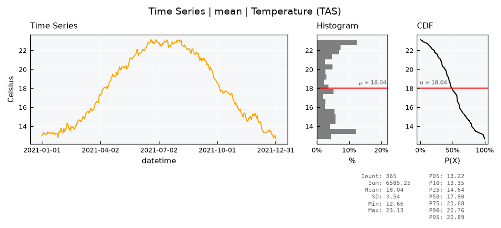
To use a reducer as a regular series, get it with .get_reducer_series(). It returns an object of the ensemble base type (here a TemperatureSeries), so all its methods are available:

ts_mean = tse.get_reducer_series(name="mean")
print(type(ts_mean))
ts_mean.view()

<class 'plans.datasets.chrono.TemperatureSeries'>

Visualizations

The default view of an ensemble draws the members in a light background style, and highlights on top the reducers listed in view_specs["reducers"] (the mean, by default) and the percentile bands in view_specs["bands"] (5 to 95, by default):

tse.view()

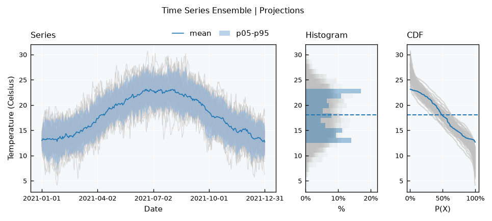
Note how narrow the histogram and the CDF of the mean are, compared to any member. Averaging cancels out the weather of individual members, so the ensemble mean is a summary of the ensemble, not a realistic realization: it has far fewer warm and cold extremes than any member.

Choosing reducers and bands

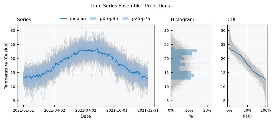
Reducers are given by name: mean, median, min, max or a percentile such as p90. Bands are given as [low, high] percentile pairs, and nest when more than one is given:

tse.view_specs["reducers"] = ["median"]
tse.view_specs["bands"] = [[5, 95], [25, 75]]
tse.view()

Highlighting members

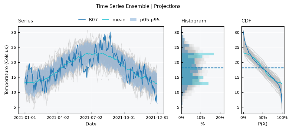
Like in a cluster, view_specs["highlight"] draws selected members in color. Compare a single member against the mean: the member is as variable as the background, while the mean is smooth:

tse.view_specs["reducers"] = ["mean"]
tse.view_specs["bands"] = [[5, 95]]
tse.view_specs["highlight"] = ["R07"]
tse.view()

For the series panel only, use the series-simple layout:

tse.view_specs["highlight"] = None
tse.view_specs["layout"] = "series-simple"
tse.view()

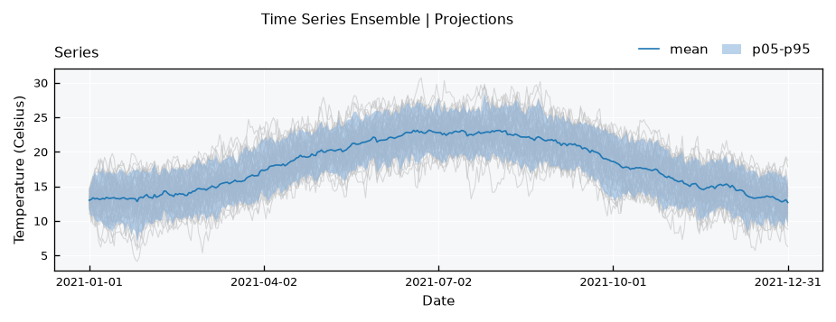
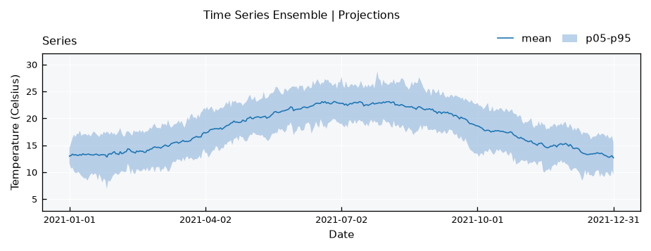
The background lines can clutter the panel, mainly with many members. Set view_specs["plot_background"] to False to hide them. This only affects the series panel, and highlighted members are still drawn:

tse.view_specs["plot_background"] = False
tse.view()

Recap

• A TimeSeriesEnsemble holds realizations of the same series, assembled like any collection.

• Reducers (.mean(), .percentiles(), .stats(), …) compute statistics across members at each time step, ignoring missing values; .reducer() takes custom functions.

• .get_reducer_series() turns a reducer into a regular series.

• The default view highlights reducers and percentile bands over the members, set by view_specs["reducers"] and view_specs["bands"].

• view_specs["plot_background"] = False hides the background lines of the series panel.