Time Series - Collections

This tutorial builds a minimal TimeSeriesCollection for one (synthetic) catchment with five sensors that deliberately differ along every axis TimeSeriesCollection has to manage:

Series	Frequency	Range	Gaps
P (rainfall)	daily	full year	1 small (3d) + 1 large (20d)
Q1 (streamflow)	daily	Mar–Nov (shorter)	1 small (2d)
Q2 (streamflow)	daily	Mar–Nov (shorter)	1 small (2d)
T (air temp.)	hourly	Jan–Jun (shorter, different unit of time)	1 small (5h) + 1 large (72h)
ET (evapotransp.)	daily	full year	2 separate medium gaps (10d, 15d)

Covered here:

• Building the four series with TimeSeries.make_synthetic_tsn()

• Loading them into one TimeSeriesCollection

• standardize() and what it does to each series

• Cross-series overlap via get_epochs()

• Per-series gap/epoch structure via merge_local_epochs()

Notebook setup

For users running this tutorial as a Jupyter Notebook, this cell must be executed first:

import sys
from pathlib import Path
import numpy as np
import pandas as pd
import matplotlib.pyplot as plt

# Install `plans` in `google.colab`.
# Use `pip install plans` for other environments.

if "google.colab" in sys.modules:
    import os
    os.system(f"{sys.executable} -m pip install -q plans")

from plans.datasets.core import TimeSeries, TimeSeriesCollection

# This avoids warnings related to uninstalled fonts
import logging
logging.getLogger('matplotlib.font_manager').setLevel(logging.ERROR)

OUTPUT_DIR = Path("outputs/time-series-collection")
OUTPUT_DIR.mkdir(parents=True, exist_ok=True)
print(f"Outputs will be saved to: ./{OUTPUT_DIR}")

RNG_SEED = 1
np.random.seed(RNG_SEED)

Outputs will be saved to: ./outputs/time-series-collection

Build synthetic series

df_p = TimeSeries.make_synthetic_tsn(
    start="2019-01-01", end="2019-12-31", base=3, trend=0.0,
    amplitude=2, noise_sd=2.5, freq="D",
    seasonal_period="YS", minor_seasonal_period="D", minor_amplitude=0,
    variable="P",
)
df_p["P"] = df_p["P"].clip(lower=0)
df_p.loc[20:22, "P"] = np.nan     # small gap (3d) -> interpolate_gaps should close this
df_p.loc[150:169, "P"] = np.nan   # large gap (20d) -> a real Epoch 0 gap

df_q = TimeSeries.make_synthetic_tsn(
    start="2019-03-01", end="2019-11-30", base=15, trend=0.01,
    amplitude=5, noise_sd=0.3, freq="D",
    seasonal_period="YS", minor_seasonal_period="D", minor_amplitude=0,
    variable="Q",
)
df_q.loc[40:41, "Q"] = np.nan     # small gap (2d)

df_q2 = TimeSeries.make_synthetic_tsn(
    start="2019-03-20", end="2019-11-30", base=15, trend=0.01,
    amplitude=5, noise_sd=0.4, freq="D",
    seasonal_period="YS", minor_seasonal_period="D", minor_amplitude=0,
    variable="Q",
)
df_q2.loc[46:50, "Q"] = np.nan     # small gap (2d)

df_t = TimeSeries.make_synthetic_tsn(
    start="2019-01-01", end="2019-06-30", base=22, trend=0.0,
    amplitude=4, noise_sd=1.5, freq="h",
    seasonal_period="YS", minor_seasonal_period="D", minor_amplitude=3,
    variable="T",
)
df_t.loc[100:104, "T"] = np.nan     # small gap (5h)
df_t.loc[2000:2071, "T"] = np.nan   # large gap (72h)

df_et = TimeSeries.make_synthetic_tsn(
    start="2019-01-01", end="2019-12-31", base=4, trend=0.0,
    amplitude=1.5, noise_sd=0.5, freq="D",
    seasonal_period="YS", minor_seasonal_period="D", minor_amplitude=0,
    variable="ET",
)
df_et["ET"] = df_et["ET"].clip(lower=0)
df_et.loc[60:69, "ET"] = np.nan     # medium gap (10d)
df_et.loc[300:314, "ET"] = np.nan   # medium gap (15d), separate from the first

for df, fname in [(df_p, "rain.csv"), (df_q, "flow.csv"), (df_q2, "flow2.csv"), (df_t, "temp.csv"), (df_et, "et.csv")]:
    df.to_csv(OUTPUT_DIR / fname, index=False, sep=";")

print("5 series written to", OUTPUT_DIR)

5 series written to outputs/time-series-collection

Load into a Time Series Collection

TimeSeriesCollection reads one info table describing every series (name, alias, file, variable/datetime columns, units, coordinates):

info = pd.DataFrame({
    "Name": ["Rain", "Flow", "Flow2", "AirTemp", "ET"],
    "Alias": ["P1", "Q1", "Q2", "T1", "ET1"],
    "File": [str(OUTPUT_DIR / f) for f in ["rain.csv", "flow.csv", "flow2.csv", "temp.csv", "et.csv"]],
    "VarField": ["P", "Q", "Q", "T", "ET"],
    "DtField": ["datetime"] * 5,
    "Units": ["mm", "m3/s", "m3/s", "C", "mm"],
    "X": [0, 0, 0, 0, 0],
    "Y": [0, 0, 0, 0, 0],
    "Code": ["P001", "Q001", "Q002", "T001", "ET001"],
    "Source": ["synthetic"] * 5,
    "Description": [
        "daily rainfall",
        "daily streamflow", "daily streamflow",
        "hourly air temperature",
        "daily evapotranspiration"
    ],
    "Color": ["tab:blue", "tab:purple", "tab:purple", "tab:red", "tab:orange"],
})
info_file = OUTPUT_DIR / "info.csv"
info.to_csv(info_file, index=False, sep=";")

tsc = TimeSeriesCollection(name="MultiSensorCatchment")
tsc.load_data(table_file=str(info_file))
tsc.catalog

	name	alias	size	color	source	description	units	code	x	y	...	datetime_res	start	end	is_standard	gap_size	n_epoch	n_gaps_small	file_data_datetime_field	file_data_variable_field	file_data
0	AirTemp	T1	4321	tab:red	synthetic	hourly air temperature	C	T001	0	0	...	hour	2019-01-01	2019-06-30	False	6	None	None	datetime	T	/home/runner/work/plans/plans/docs/tutorials/o...
1	ET	ET1	365	tab:orange	synthetic	daily evapotranspiration	mm	ET001	0	0	...	day	2019-01-01	2019-12-31	False	6	None	None	datetime	ET	/home/runner/work/plans/plans/docs/tutorials/o...
2	Flow	Q1	275	tab:purple	synthetic	daily streamflow	m3/s	Q001	0	0	...	day	2019-03-01	2019-11-30	False	6	None	None	datetime	Q	/home/runner/work/plans/plans/docs/tutorials/o...
3	Flow2	Q2	256	tab:purple	synthetic	daily streamflow	m3/s	Q002	0	0	...	day	2019-03-20	2019-11-30	False	6	None	None	datetime	Q	/home/runner/work/plans/plans/docs/tutorials/o...
4	Rain	P1	365	tab:blue	synthetic	daily rainfall	mm	P001	0	0	...	day	2019-01-01	2019-12-31	False	6	None	None	datetime	P	/home/runner/work/plans/plans/docs/tutorials/o...

5 rows × 29 columns

Raw series at a glance

Visualize individual TimeSeries accessing by the name

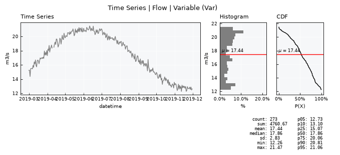
tsc.collection["Flow"].view()
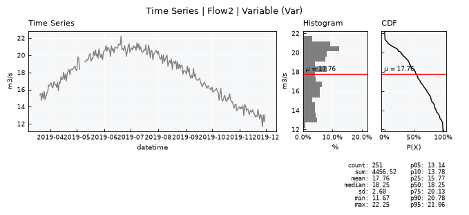
tsc.collection["Flow2"].view()

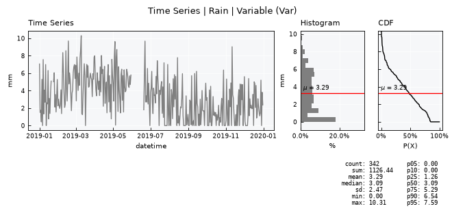
tsc.collection["Rain"].view()
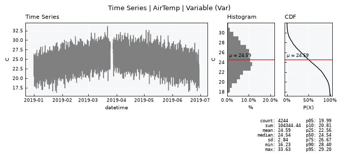
tsc.collection["AirTemp"].view()
tsc.collection["ET"].view()

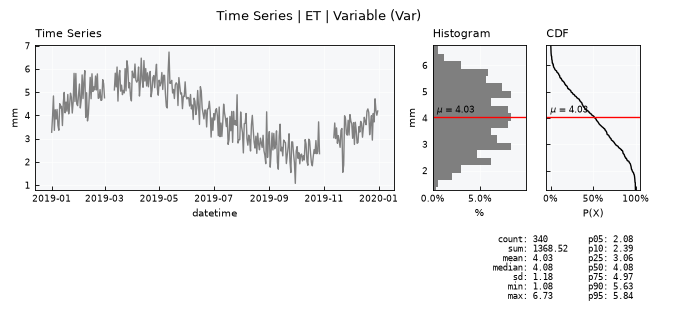
Learn about the epochs

Visualize epochs per Time Series

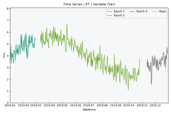
tsc.collection["ET"].view_epochs()

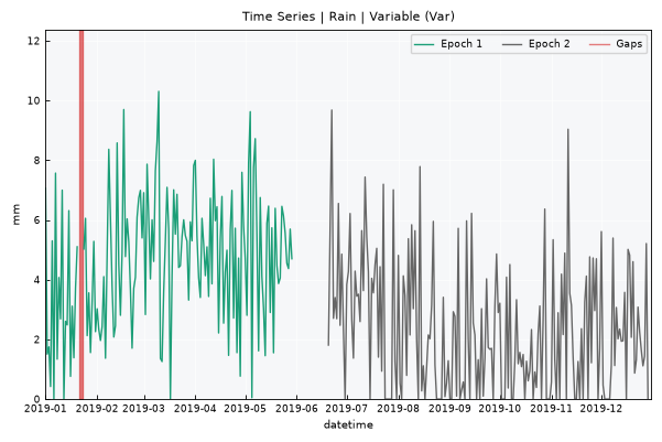
tsc.collection["Rain"].view_epochs()

Learn collection-wise epochs

df_local_epochs = tsc.merge_local_epochs()
df_local_epochs

	name	id_epoch	n_epoch	n_gaps_small	start	end	color
0	Rain	1	150	3	2019-01-01 00:00:00	2019-05-30 00:00:00	#1b9e77
1	Rain	2	194	0	2019-06-20 00:00:00	2019-12-30 00:00:00	#666666
2	Flow	1	274	2	2019-03-01 00:00:00	2019-11-29 00:00:00	#1b9e77
3	Flow2	1	255	5	2019-03-20 00:00:00	2019-11-29 00:00:00	#1b9e77
4	AirTemp	1	2000	5	2019-01-01 00:00:00	2019-03-25 07:00:00	#1b9e77
5	AirTemp	2	2248	0	2019-03-28 08:00:00	2019-06-29 23:00:00	#666666
6	ET	1	60	0	2019-01-01 00:00:00	2019-03-01 00:00:00	#1b9e77
7	ET	2	230	0	2019-03-12 00:00:00	2019-10-27 00:00:00	#66a61e
8	ET	3	49	0	2019-11-12 00:00:00	2019-12-30 00:00:00	#666666

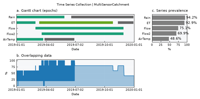
Visualize collection-wise epochs

tsc.view()

Get merged data epochs

tsc.get_epochs()

	datetime	v_T1	v_ET1	v_Q1	v_Q2	v_P1	Overlapping	id_epoch
0	2019-01-01 00:00:00	20.558105	3.278440	NaN	NaN	7.060863	0.6	1
1	2019-01-01 01:00:00	20.591839	NaN	NaN	NaN	NaN	0.2	1
2	2019-01-01 02:00:00	24.247251	NaN	NaN	NaN	NaN	0.2	1
3	2019-01-01 03:00:00	21.888637	NaN	NaN	NaN	NaN	0.2	1
4	2019-01-01 04:00:00	23.939504	NaN	NaN	NaN	NaN	0.2	1
...	...	...	...	...	...	...	...	...
4500	2019-12-27 00:00:00	NaN	3.721585	NaN	NaN	1.434334	0.4	5
4501	2019-12-28 00:00:00	NaN	4.716271	NaN	NaN	5.210317	0.4	5
4502	2019-12-29 00:00:00	NaN	4.225181	NaN	NaN	0.000000	0.4	5
4503	2019-12-30 00:00:00	NaN	4.009106	NaN	NaN	3.812393	0.4	5
4504	2019-12-31 00:00:00	NaN	4.192162	NaN	NaN	2.374481	0.4	0

4505 rows × 8 columns

Standardize collection

Regularizes each series onto its own regular time step and closes small gaps (interpolate_gaps), then merges all series onto one shared table:

tsc.standardize()

for name in tsc.collection:
    d = tsc.collection[name]
    print(f"{name:>10}: n={len(d.data):5d}  nan={d.data['v'].isna().sum():5d}  "
          f"freq={d.dtfreq:>3}  start={d.start.date()}  end={d.end.date()}")

      Rain: n=  367  nan=   21  freq=  D  start=2019-01-01  end=2020-01-02
      Flow: n=  277  nan=    1  freq=  D  start=2019-03-01  end=2019-12-02
     Flow2: n=  258  nan=    1  freq=  D  start=2019-03-20  end=2019-12-02
   AirTemp: n= 4369  nan=   73  freq=  h  start=2019-01-01  end=2019-07-02
        ET: n=  367  nan=   26  freq=  D  start=2019-01-01  end=2020-01-02

Merge data

The .merge_data() is a helper method that makes an outer join for the available time series, returning a dataframe with all the data.

df_merged = tsc.merge_data()
df_merged

	datetime	v_T1	v_ET1	v_Q1	v_Q2	v_P1
0	2019-01-01 00:00:00	20.558105	3.278440	NaN	NaN	7.060863
1	2019-01-01 01:00:00	20.591839	NaN	NaN	NaN	NaN
2	2019-01-01 02:00:00	24.247251	NaN	NaN	NaN	NaN
3	2019-01-01 03:00:00	21.888637	NaN	NaN	NaN	NaN
4	2019-01-01 04:00:00	23.939504	NaN	NaN	NaN	NaN
...	...	...	...	...	...	...
4548	2019-12-29 00:00:00	NaN	4.225181	NaN	NaN	0.000000
4549	2019-12-30 00:00:00	NaN	4.009106	NaN	NaN	3.812393
4550	2019-12-31 00:00:00	NaN	4.192162	NaN	NaN	2.374481
4551	2020-01-01 00:00:00	NaN	4.375219	NaN	NaN	0.936569
4552	2020-01-02 00:00:00	NaN	NaN	NaN	NaN	NaN

4553 rows × 6 columns

Recap

• Built 5 synthetic series with independently varied range, gap structure, and time step.

• TimeSeriesCollection.load_data() reads them all from one info table into a shared catalog.

• get_epochs() / merge_local_epochs() give the cross-series and per-series gap/epoch pictures respectively.