Time Series - Clusters

A TimeSeriesCluster holds series of the same variable from different sites, like a network of weather stations or rain gauges. Unlike a TimeSeriesCollection, which accepts miscellaneous data, a cluster can compare its series against each other: how correlated the sites are, and how one site can fill the gaps of another.

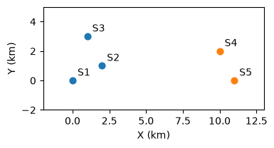
This tutorial builds a synthetic network of five temperature stations in two sub-regions:

Station	Sub-region	Range	Gaps
S1	west	full year	1 large (30d)
S2	west	full year	none
S3	west	full year	none
S4	east	Mar-Dec (shorter)	none
S5	east	full year	1 small (3d)

Covered here:

• Loading the stations into a TemperatureSeriesCluster

• Viewing data availability and all series together

• Correlation between stations via get_correlation()

• Gap filling from other stations via regionalize(), comparing uniform and inverse-distance weights

See also

Check out the Time Series - Collections tutorial first.

Notebook setup

For users running this tutorial as a Jupyter Notebook, this cell must be executed first:

import sys
import copy
from pathlib import Path
import numpy as np
import pandas as pd
import matplotlib.pyplot as plt

# Install `plans` in `google.colab`.
# Use `pip install plans` for other environments.

if "google.colab" in sys.modules:
    import os
    os.system(f"{sys.executable} -m pip install -q plans")

from plans.datasets import TemperatureSeriesCluster
from plans.datasets.analyst import Bivar

# This avoids warnings related to uninstalled fonts
import logging
logging.getLogger('matplotlib.font_manager').setLevel(logging.ERROR)

OUTPUT_DIR = Path("outputs/time-series-cluster")
OUTPUT_DIR.mkdir(parents=True, exist_ok=True)
print(f"Outputs will be saved to: ./{OUTPUT_DIR}")

rng = np.random.default_rng(seed=7)  # ensure reproducibility

Outputs will be saved to: ./outputs/time-series-cluster

Build a synthetic station network

Each station gets the same cycle, a weather anomaly common to the whole region, a weather anomaly of its own sub-region, and some local shocks. The anomalies have memory (an autoregressive process), so warm or cold spells last for some days. Stations in the same sub-region share more signal, so they should correlate more.

n = 365
t = np.arange(n)

def make_anomaly(phi, sd):
    # autoregressive anomaly: a[t] = phi * a[t-1] + shock
    a = np.zeros(n)
    e = rng.normal(loc=0, scale=sd, size=n)
    for i in range(1, n):
        a[i] = phi * a[i - 1] + e[i]
    return a

cycle = 18 + 4 * np.sin(2 * np.pi * (t - 100) / 365)
anomaly_region = make_anomaly(phi=0.8, sd=1.0)
anomaly_subregion = {
    "west": make_anomaly(phi=0.8, sd=1.2),
    "east": make_anomaly(phi=0.8, sd=1.2),
}

# stations: sub-region and coordinates (km)
stations = pd.DataFrame({
    "Name": ["S1", "S2", "S3", "S4", "S5"],
    "Subregion": ["west", "west", "west", "east", "east"],
    "X": [0, 2, 1, 10, 11],
    "Y": [0, 1, 3, 2, 0],
})

dates = pd.date_range(start="2021-01-01", periods=n, freq="D")
dc_series = {}
for _, row in stations.iterrows():
    dc_series[row["Name"]] = (
        cycle
        + anomaly_region
        + anomaly_subregion[row["Subregion"]]
        + rng.normal(loc=0, scale=0.8, size=n)
    )

Lets look at where the stations are:

fig, ax = plt.subplots(figsize=(4, 3))
colors = {"west": "tab:blue", "east": "tab:orange"}
for _, row in stations.iterrows():
    ax.scatter(row["X"], row["Y"], color=colors[row["Subregion"]], s=40)
    ax.annotate(row["Name"], (row["X"], row["Y"]), xytext=(5, 5), textcoords="offset points")
ax.set_xlim(-2, 13)
ax.set_ylim(-2, 5)
ax.set_aspect("equal")
ax.set_xlabel("X (km)")
ax.set_ylabel("Y (km)")
plt.show()

Now add the gaps. Before removing the values of the large gap in S1, keep them as the truth, so we can later check how well the gap was filled:

# large gap in S1 -- keep the truth
GAP = slice(150, 180)
truth = dc_series["S1"][GAP].copy()
dc_series["S1"][GAP] = np.nan

# small gap in S5
dc_series["S5"][200:203] = np.nan

# save files -- S4 starts later
ls_files = []
for name, values in dc_series.items():
    df = pd.DataFrame({"datetime": dates, "T": values})
    if name == "S4":
        df = df.iloc[60:]
    file = OUTPUT_DIR / f"{name}.csv"
    df.to_csv(file, sep=";", index=False)
    ls_files.append(str(file))
print(ls_files)

['outputs/time-series-cluster/S1.csv', 'outputs/time-series-cluster/S2.csv', 'outputs/time-series-cluster/S3.csv', 'outputs/time-series-cluster/S4.csv', 'outputs/time-series-cluster/S5.csv']

Load into a Time Series Cluster

Like a collection, a cluster is loaded from an info table. The X and Y columns are the station coordinates, used later for inverse-distance weights. Here we use TemperatureSeriesCluster, a cluster ready for temperature series:

info = pd.DataFrame({
    "Name": stations["Name"],
    "Alias": stations["Name"],
    "File": ls_files,
    "VarField": "T",
    "DtField": "datetime",
    "Units": "C",
    "X": stations["X"],
    "Y": stations["Y"],
    "Code": stations["Name"],
    "Source": "synthetic",
    "Description": "daily air temperature, " + stations["Subregion"] + " sub-region",
    "Color": "tab:red",
})
info_file = OUTPUT_DIR / "info.csv"
info.to_csv(info_file, sep=";", index=False)

tsc = TemperatureSeriesCluster(name="Network")
tsc.load_data(table_file=info_file)
tsc.catalog[["name", "x", "y", "start", "end", "variable_min", "variable_max"]]

	name	x	y	start	end	variable_min	variable_max
0	S1	0	0	2021-01-01	2021-12-31	7.014798	27.477313
1	S2	2	1	2021-01-01	2021-12-31	8.057301	27.454874
2	S3	1	3	2021-01-01	2021-12-31	8.387260	26.842874
3	S4	10	2	2021-03-02	2021-12-31	8.225353	26.716260
4	S5	11	0	2021-01-01	2021-12-31	7.162614	25.622818

Data availability

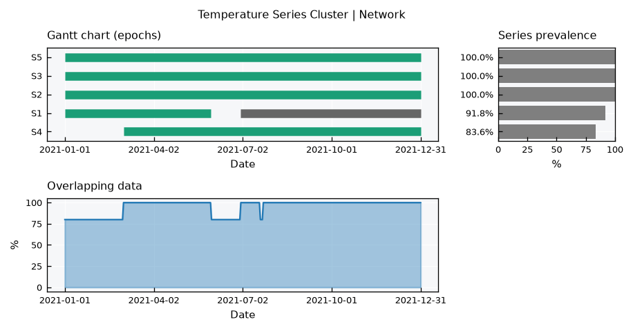
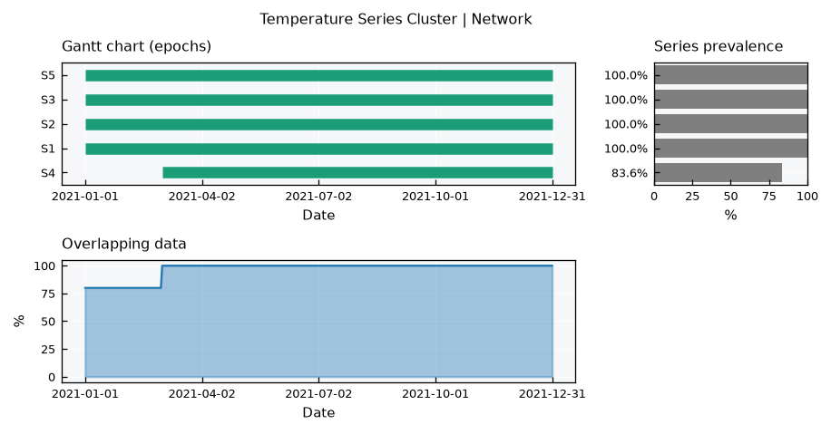
The default .view() is inherited from the collection: the Gantt chart of each series epochs, the overlapping data across series, and the series prevalence. Note the gap in S1 and the late start of S4:

tsc.view()

All series together

Since all series are the same variable, they can share the same axes. The series layout mirrors the single TimeSeries view, overlaying every station: the series, their histograms (with common bins) and their CDFs, with dashed lines for the means:

tsc.view_specs["layout"] = "series"
tsc.view()

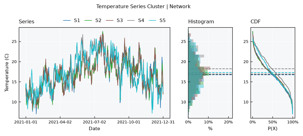
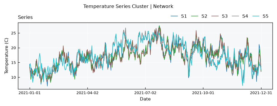
The cycle dominates, but the two sub-regions drift apart during warm and cold spells. Note also that S4 has a higher mean: its record starts in March, missing the coldest months. Comparing statistics between sites requires a common period.

For the series only, use the series-simple layout:

tsc.view_specs["layout"] = "series-simple"
tsc.view()

Correlation between stations

The .get_correlation() method computes the correlation matrix between all stations, using only the time steps where both have data. Pairs with fewer overlapping steps than min_overlap are set to NaN:

df_corr = tsc.get_correlation(method="pearson", min_overlap=30)
df_corr.round(3)

	S1	S2	S3	S4	S5
S1	1.000	0.952	0.952	0.644	0.690
S2	0.952	1.000	0.953	0.607	0.673
S3	0.952	0.953	1.000	0.617	0.685
S4	0.644	0.607	0.617	1.000	0.961
S5	0.690	0.673	0.685	0.961	1.000

Use the correlation layout to see it as a heatmap:

tsc.view_specs["layout"] = "correlation"
tsc.view()

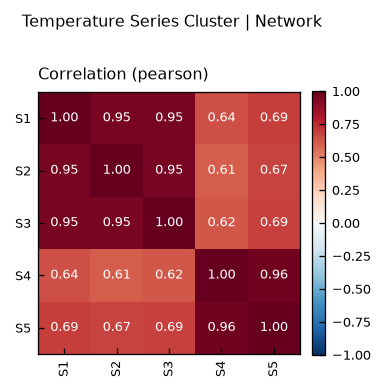
The two sub-regions show up as two blocks: stations of the same sub-region correlate around 0.95, while stations of different sub-regions stay around 0.7. Spearman correlation is also available with method="spearman".

Note

With a strong cycle, correlation is partly driven by the shared cycle itself. Even unrelated sites under the same climate correlate well.

Filling gaps from other stations

The .regionalize() method fills the gaps of every station with a weighted average of the other stations, on the time steps where they have data. Observed values are never changed. Two weighting methods are available:

• average: all other stations get the same weight.

• idw: inverse distance weighting, closer stations get more weight.

Check the share of each station in the weights for S1:

df_weights = pd.DataFrame(
    {method: tsc.get_weights_by_name(name="S1", method=method) for method in ["average", "idw"]},
    index=["S2", "S3", "S4", "S5"],
)
df_weights = df_weights / df_weights.sum()
df_weights.round(2)

	average	idw
S2	0.25	0.47
S3	0.25	0.33
S4	0.25	0.10
S5	0.25	0.10

Since .regionalize() changes the data in place, lets run each method on a copy of the cluster:

dc_clusters = {}
for method in ["average", "idw"]:
    dc_clusters[method] = copy.deepcopy(tsc)
    dc_clusters[method].regionalize(method=method)

The gap in S1 is now closed:

tsc_idw = dc_clusters["idw"]
tsc_idw.view_specs["layout"] = "full"
tsc_idw.view()

How good is the filling?

Since we kept the truth, we can compare the filled values against it using the Bivar metrics:

gap_dates = dates[GAP]
dc_filled = {}
for method, cluster in dc_clusters.items():
    ts = cluster.collection["S1"]
    s = ts.data.set_index(ts.dtfield)[ts.varfield]
    dc_filled[method] = s.loc[gap_dates].values

df_metrics = pd.DataFrame(
    {method: Bivar.get_metrics(observed=truth, predicted=filled) for method, filled in dc_filled.items()}
).T
df_metrics[["RMSE", "MAE", "Bias", "R2"]]

	RMSE	MAE	Bias	R2
average	1.952558	1.547067	7.487313	0.022263
idw	1.040685	0.824099	2.649993	0.722251

And see it on the gap window:

fig, ax = plt.subplots(figsize=(7, 3))
ax.plot(gap_dates, truth, color="black", label="truth")
ax.plot(gap_dates, dc_filled["average"], color="tab:gray", linestyle="--", label="average")
ax.plot(gap_dates, dc_filled["idw"], color="tab:blue", label="idw")
ax.set_ylabel("Temperature (C)")
ax.legend(frameon=False)
plt.show()

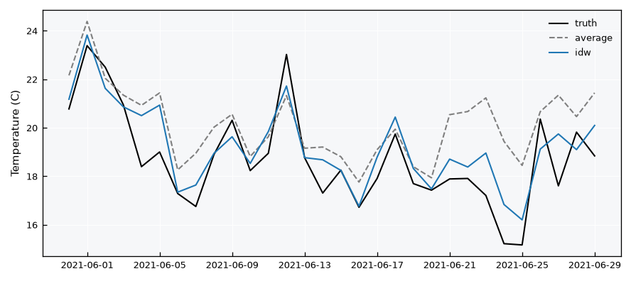
Inverse distance weighting follows the truth much closer, since it relies mostly on S2 and S3, which share the west sub-region weather. The uniform average gives half of the weight to the east stations, which have their own weather.

Warning

.regionalize() takes the other stations values as they are. Stations with systematically different levels (e.g., temperature at different elevations) will bias the filling.

Recap

• A TimeSeriesCluster holds same-variable series from different sites, loaded from an info table with station coordinates.

• The series and correlation layouts show the series together and the correlation between sites; the default layout shows data availability.

• get_correlation() compares sites on their overlapping time steps.

• regionalize() fills gaps from other sites, with uniform or inverse-distance weights.