Time Series - Comparing

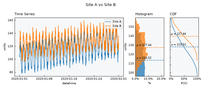
It’s common to want a quick visual comparison between two time series – two sensors, two sites, before/after a data-cleaning step, and so on. TimeSeries.view_compare_times_series() is a static method that overlays two TimeSeries objects on a shared time axis, alongside a histogram and CDF, so their distributions can be compared at a glance.

Covered here:

• Loading two independent TimeSeries objects

• Calling view_compare_times_series() inline (return_fig=True)

• Setting per-series colors via view_specs

• Saving the comparison to a file instead of displaying it inline

Notebook setup

For users running this tutorial as a Jupyter Notebook, this cell must be executed first:

import sys
from pathlib import Path
import numpy as np
import pandas as pd
import matplotlib.pyplot as plt

# Install `plans` in `google.colab`.
# Use `pip install plans` for other environments.

if "google.colab" in sys.modules:
    import os
    os.system(f"{sys.executable} -m pip install -q plans")

# This avoids warnings related to uninstalled fonts
import logging
logging.getLogger('matplotlib.font_manager').setLevel(logging.ERROR)

# define output folder
OUTPUT_DIR = Path("outputs/time-series")
OUTPUT_DIR.mkdir(parents=True, exist_ok=True)
print(f"Outputs will be saved to: ./{OUTPUT_DIR}")

RNG_SEED = 1
np.random.seed(RNG_SEED)

Outputs will be saved to: ./outputs/time-series

Create two synthetic series to compare

Two Trend-Seasonality-Noise archetype series with different bases, trends, and noise levels – a stand-in for, e.g., two different sensors or sites over the same period.

from plans.datasets import TimeSeries

df_site_a = TimeSeries.make_synthetic_tsn(
    start="2020-01-01",
    end="2020-02-01",
    base=100,
    freq="1h",
    trend=0.001,
    noise_sd=4.0,
    amplitude=50,
    seasonal_period="YS",
    minor_amplitude=20,
    minor_seasonal_period="D"
)

df_site_b = TimeSeries.make_synthetic_tsn(
    start="2020-01-01",
    end="2020-02-01",
    base=120,
    freq="1h",
    trend=-0.002,
    noise_sd=6.0,
    amplitude=30,
    seasonal_period="YS",
    minor_amplitude=15,
    minor_seasonal_period="D"
)

print(f"Site A rows: {len(df_site_a)}")
print(f"Site B rows: {len(df_site_b)}")

Site A rows: 745
Site B rows: 745

Save and load both as TimeSeries objects

file_a = OUTPUT_DIR / "site_a.csv"
file_b = OUTPUT_DIR / "site_b.csv"
df_site_a.to_csv(file_a, sep=";", index=False)
df_site_b.to_csv(file_b, sep=";", index=False)

ts_a = TimeSeries(name="Site A", alias="a")
ts_a.load_data(
    file_data=file_a,
    input_dtfield="datetime",
    input_varfield="level",
    in_sep=";",
)

ts_b = TimeSeries(name="Site B", alias="b")
ts_b.load_data(
    file_data=file_b,
    input_dtfield="datetime",
    input_varfield="level",
    in_sep=";",
)

Comparing the two series

view_compare_times_series() is a static method on TimeSeries – called on the class itself, not an instance – taking both series plus a specs dict of plot overrides. It draws:

• the two series overlaid on a shared time axis (left panel)

• a horizontal histogram of each series’ distribution (middle panel)

• a CDF with each series’ mean annotated (right panel)

Each series keeps its own color, set via view_specs["color"] on each object before calling the method, and its own label, taken from .name.

ts_a.view_specs["color"] = "tab:blue"
ts_b.view_specs["color"] = "tab:orange"
ts_a.view_specs["n_dates"] = 5

specs = {"title": "Site A vs Site B"}

fig = TimeSeries.view_compare_times_series(
    ts_a, ts_b, specs, return_fig=True
)
plt.show()

Saving to a file

With return_fig=False (the default), the method saves the figure to disk instead of returning it. In that mode, specs must also include "folder" and "filename" – these are used to build the output path ("{folder}/{filename}.{fig_format}"). Note that dpi and fig_format are not read from specs; they’re always taken from ts_first.view_specs regardless of what’s passed.

specs_save = {
    "title": "Site A vs Site B",
    "folder": str(OUTPUT_DIR),
    "filename": "site_a_vs_site_b",
}

TimeSeries.view_compare_times_series(
    ts_a, ts_b, specs_save, show=False, return_fig=False
)

saved_path = OUTPUT_DIR / f"site_a_vs_site_b.{ts_a.view_specs['fig_format']}"
print(f"Saved to: {saved_path}")
print(f"Exists: {saved_path.exists()}")

Saved to: outputs/time-series/site_a_vs_site_b.jpg
Exists: True

Note: view_specs is mutated in place

Both ts_a.view_specs and ts_b.view_specs are updated in place by the call above – the contents of specs get merged in, along with layout and color settings the method sets internally. If you plan to call .view() on either series afterward expecting its original single-series layout, be aware the specs have changed:

print(f"ts_a.view_specs['title'] after comparison call: {ts_a.view_specs['title']!r}")
print(f"ts_a.view_specs['layout'] after comparison call: {ts_a.view_specs['layout']!r}")

ts_a.view_specs['title'] after comparison call: 'Site A vs Site B'
ts_a.view_specs['layout'] after comparison call: 'mini'

Recap

• TimeSeries.view_compare_times_series(ts1, ts2, specs, ...) is a static method that overlays two series with a shared histogram/CDF comparison.

• Set each series’ view_specs["color"] beforehand to control which color it’s plotted in; the label comes from .name.

• Use return_fig=True for inline display (e.g. in a notebook); omit it (or set False) to save to "{folder}/{filename}.{fig_format}", in which case specs must include "folder" and "filename".

• Both input objects’ view_specs are mutated in place by the call – pass copies if you need the originals preserved for later single-series .view() calls.